An Intuitive Guide to Interpret a Random Forest Model using fastai library (Machine Learning for Programmers – Part 2)

Introduction

Machine Learning is a fast evolving field – but a few things would remain as they were years ago. One such thing is ability to interpret and explain your machine learning models. If you build a model and can not explain it to your business users – it is very unlikely that it will see the light of the day.

Can you imagine integrating a model into your product without understanding how it works? Or which features are impacting your final result?

In addition to backing from stakeholders, we as data scientists benefit from interpreting our work and improving upon it. It’s a win-win situation all around!

The first article of this fast.ai machine learning course saw an incredible response from our community. I’m delighted to share part 2 of this series, which primarily deals with how you can interpret a random forest model. We will understand the theory and also implement it in Python to solidify our grasp on this critical concept.

As always, I encourage you to replicate the code on your own machine while you go through the article. Experiment with the code and see how different your results are from what I have covered in this article. This will help you understand the different facets of both the random forest algorithm and the importance of interpretability.

Table of contents

1. Overview of Part 1 (Lessons 1 and 2)
2. Introduction to Machine Learning : Lesson 3
   2.1 Building a Random Forest
   2.2 Confidence Based on Tree Variance
   2.3 Feature Importance
3. Introduction to Machine learning : Lesson 4
   3.1 One Hot Encoding
   3.2 Removing Redundant features
   3.3 Partial Dependence
   3.4 Tree Interpreter
4. Introduction to Machine Learning : Lesson 5
   4.1 Extrapolation
   4.2 Random Forest from scratch
5. Additional Topics

Overview of Part 1 (Lessons 1 and 2)

Before we dive into the next lessons of this course, let’s quickly recap what we covered in the first two lessons. This will give you some context as to what to expect moving forward.

• Data exploration and preprocessing : Explored the bulldozer dataset (link), imputed missing values and converted the categorical variables into numeric columns that are accepted by the ml models. We also created multiple features from the date column using date_part function from fastai library.
• Building a Random Forest model and creating a validation set: We implemented a random forest and calculated the score on the train set. In order to make sure that the model is not overfitting, a validation set was created. Further we tuned the parameters to improve the performance of the model.
• Introduction to Bagging: The concept of bagging was introduced in the second video. We also visualized a single tree that provided a better understanding about how random forests work.

We will continue working on the same dataset in this article. We will have a look at what are the different variables in the dataset and how can we build a random forest model to make valuable interpretations.

Alright, it’s time to fire up our Jupyter notebooks and dive right in to lesson#3!

Introduction to Machine Learning: Lesson 3

You can access the notebook for this lesson here. This notebook will be used for all the three lessons covered in this video. You can watch the entire lesson in the below video (or just scroll down and start implementing things right away):

NOTE: Jeremy Howard regularly provides various tips that can be used for solving a certain problem more efficiently, as we saw in the previous article as well. A part of this video is about how to deal with very large datasets. I have included this in the last section of the article so we can focus on the topic at hand first.

Let’s continue from where we left off at the end of lesson 2. We had created new features using the date column and dealt with the categorical columns as well. We will load the processed dataset which includes our newly engineered features and the log of the saleprice variable (since the evaluation metric is RMSLE):

#importing necessary libraries
%load_ext autoreload
%autoreload 2
%matplotlib inline

from fastai.imports import *
from fastai.structured import *
from pandas_summary import DataFrameSummary
from sklearn.ensemble import RandomForestRegressor, RandomForestClassifier
from IPython.display import display
from sklearn import metrics

#loading preprocessed file
PATH = "data/bulldozers/"

df_raw = pd.read_feather('tmp/bulldozers-raw')
df_trn, y_trn, nas = proc_df(df_raw, 'SalePrice')

We will define the necessary functions which we’ll be frequently using throughout our implementation.

#creating a validation set

def split_vals(a,n): return a[:n], a[n:]
n_valid = 12000
n_trn = len(df_trn)-n_valid
X_train, X_valid = split_vals(df_trn, n_trn)
y_train, y_valid = split_vals(y_trn, n_trn)
raw_train, raw_valid = split_vals(df_raw, n_trn)

#define function to calculate rmse and print score
def rmse(x,y): return math.sqrt(((x-y)**2).mean())

def print_score(m):
   res = [rmse(m.predict(X_train), y_train), rmse(m.predict(X_valid), y_valid),
               m.score(X_train, y_train), m.score(X_valid, y_valid)]
   if hasattr(m, 'oob_score_'): res.append(m.oob_score_)
   print(res)

The next step will be to implement a random forest model and interpret the results to understand our dataset better. We have so far learned that random forest is a group of many trees, each trained on a different subset of data points and features. Each individual tree is as different as possible, capturing unique relations from the dataset. We make predictions by running each row through each tree and taking the average of the values at the leaf node. This average is taken as the final prediction for the row.

While interpreting the results, it is necessary that the process is interactive and takes lesser time to run. To make this happen, we will make two changes in the code (as compared to what we implemented in the previous article):

1.  Take a subset of the data:

set_rf_samples(50000)

We’re only using a sample as working with the entire data will take a long time to run. An important thing to note here is that the sample should not be very small. This might end up giving a different result and that’ll be detrimental to our entire project. A sample size of 50,000 works well.

#building a random forest model

m = RandomForestRegressor(n_estimators=40, min_samples_leaf=3, max_features=0.5, n_jobs=-1, oob_score=True)
m.fit(X_train, y_train)
print_score(m)

2. Make predictions in parallel

Previously, we made predictions for each row using every single tree and then we calculated the mean of the results and the standard deviation.

%time preds = np.stack([t.predict(X_valid) for t in m.estimators_])
np.mean(preds[:,0]), np.std(preds[:,0])

CPU times: user 1.38 s, sys: 20 ms, total: 1.4 s
Wall time: 1.4 s

You might have noticed that this works in a sequential manner. Instead, we can call the predict function on multiple trees in parallel! This can be achieved using the parallel_trees function in the fastai library.

def get_preds(t): return t.predict(X_valid)
%time preds = np.stack(parallel_trees(m, get_preds))
np.mean(preds[:,0]), np.std(preds[:,0])

The time taken here is less and the results are exactly the same! We will now create a copy of the data so that any changes we make do not affect the original dataset.

x = raw_valid.copy()

Once we have the predictions, we can calculate the RMSLE to determine how well the model is performing. But the overall value does not help us identify how close the predicted values are for a particular row or how confident we are that the predictions are correct. We will look at the standard deviation for the rows in this case.

If a row is different from those present in the train set, each tree will give different values as predictions. This consequently means means that the standard deviation will be high. On the other hand, the trees would make almost similar predictions for a row that is quite similar to the ones present in the train set, t, i.e., the standard deviation will be low. So, based on the value of the standard deviations we can decide how confident we are about the predictions.

Let’s save these predictions and standard deviations:

x['pred_std'] = np.std(preds, axis=0)
x['pred'] = np.mean(preds, axis=0)

Confidence based on Tree Variance

Now, let’s take up a variable from the dataset and visualization it’s distribution and understand what it actually represents. We’ll begin with the Enclosure variable.

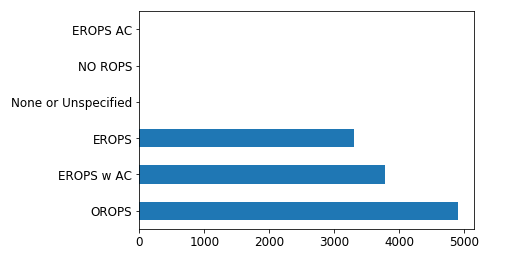
1.  Figuring out the value count of each category present in the variable Enclosure:

x.Enclosure.value_counts().plot.barh()

2. For each category, below are the mean values of saleprice, prediction and standard deviation.

flds = ['Enclosure', 'SalePrice', 'pred', 'pred_std']
enc_summ = x[flds].groupby('Enclosure', as_index=False).mean()
enc_summ

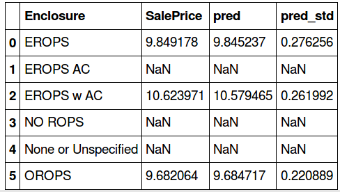
The actual sale price and the prediction values are almost similar in three categories – ‘EROPS’, ‘EROPS w AC’, ‘OROPS’ (the remaining have null values). Since these null value columns do not add any extra information, we will drop them and visualize the plots for salesprice and prediction:

enc_summ = enc_summ[~pd.isnull(enc_summ.SalePrice)]
enc_summ.plot('Enclosure', 'pred', 'barh', xerr='pred_std', alpha=0.6, xlim=(0,11));

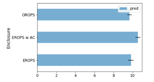
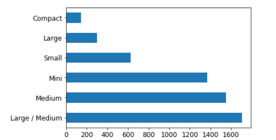
Note that the small black bars represent standard deviation. In the same way, let’s look at another variable – ProductSize.

#the value count for each category
raw_valid.ProductSize.value_counts().plot.barh();

#category wise mean for sale price, prediction and standard deviation
flds = ['ProductSize', 'SalePrice', 'pred', 'pred_std']
summ = x[flds].groupby(flds[0]).mean()
summ

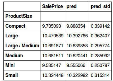
We will take a ratio of the standard deviation values and the sum of predictions in order to compare which category has a higher deviation.

(summ.pred_std/summ.pred).sort_values(ascending=False)

ProductSize
Large             0.034871
Compact           0.034297
Small             0.030545
Large / Medium    0.027799
Medium            0.026928
Mini              0.026247
dtype: float64

The standard deviation is higher for the ‘Large’ and ‘Compact’ categories. Why do you that is? Take a moment to ponder the answer before reading on.

Have a look at the bar plot of values for each category in ProductSize. Found the reason? We have a lesser number of rows for these two categories. Thus, the model is giving a relatively poor prediction accuracy for these variables.

Using this information, we can say that we are more confident about the predictions for the mini, medium and medium/large product size, and less confident about the small, compact and large ones.

Feature Importance

Feature importance is one of the key aspects of a machine learning model. Understanding which variable is contributing the most to a model is critical to interpreting the results. This is what data scientists strive for when building models that need to be explained to non-technical stakeholders.

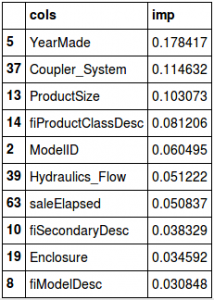
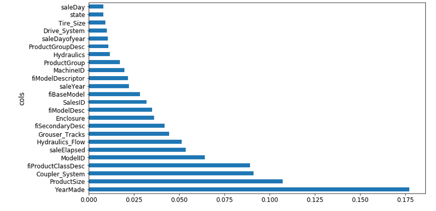
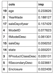
Our dataset has multiple features and it is often difficult to understand which feature is dominant. This is where the feature importance function of random forest is so helpful. Let’s look at the top 10 most important features for our current model (including visualizing them by their importance):

fi = rf_feat_importance(m, df_trn)
fi[:10]

fi.plot('cols', 'imp', figsize=(10,6), legend=False);

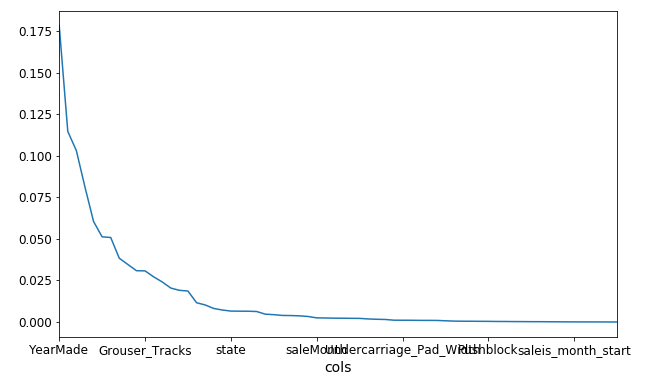
That’s a pretty intuitive plot. Here’s a bar plot visualization of the top 30 features:

def plot_fi(fi):
return fi.plot('cols','imp','barh', figsize=(12,7), legend=False)
plot_fi(fi[:30]);

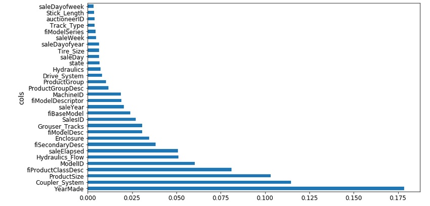
Clearly YearMade is the most important feature, followed by Coupler_System. The majority of the features seems to have little importance in the final model. Let’s verify this statement by removing these features and checking whether this affects the model’s performance.

So, we will build a random forest model using only the features that have a feature importance greater than 0.005:

to_keep = fi[fi.imp>0.005].cols
len(to_keep)

24

df_keep = df_trn[to_keep].copy()
X_train, X_valid = split_vals(df_keep, n_trn)

m = RandomForestRegressor(n_estimators=40, min_samples_leaf=3, max_features=0.5,
n_jobs=-1, oob_score=True)
m.fit(X_train, y_train)
print_score(m)

[0.20685390156773095, 0.24454842802383558, 0.91015213846294174, 0.89319840835270514, 0.8942078920004991]

When you think about it, removing redundant columns should not decrease the model score, right? And in this case, the model performance has slightly improved. Some of the features we dropped earlier might have been highly collinear with others, so removing them did not affect the model adversely. Let’s check feature importance again to verify our hypothesis:

fi = rf_feat_importance(m, df_keep)
plot_fi(fi)

The difference between the feature importance of the YearMade and Coupler_System variables is more significant. From the list of features removed, some features were highly collinear to YearMade, resulting in distribution of feature importance between them.

On removing these features, we can see that the difference between the importance of YearMade and CouplerSystem has increased from the previous plot. Here is a detailed explanation of how feature importance is actually calculated:

• Calculate the r-square considering all the columns: Suppose in this case it comes out to be 0.89
• Now randomly shuffle the values for any one column, say YearMade. This column has no relation to the target variable
• Calculate the r-square again: The r-square has dropped to 0.8. This shows that the YearMade variable is an important feature
• Take another variable, say Enclosure, and shuffle it randomly
• Calculate the r-square:  Now let’s say the r-square is coming to be 0.84. This indicates that the variable is important but comparatively less so than the YearMade variable

And that wraps up the implementation of lesson #3! I encourage you to try out these codes and experiment with them on your own machine to truly understand how each aspect of a random forest model works.

Introduction to Machine Learning : Lesson 4

In this lesson, Jeremy Howard gives a quick overview of lesson 3 initially before introducing a few important concepts like One Hot Encoding, Dendrogram, and Partial Dependence. Below is the YouTube video of the lecture (or you can jump straight to the implementation below):

One-Hot Encoding

In the first article of the series, we learned that a lot of machine learning models cannot deal with categorical variables. Using proc_df, we converted the categorical variables into numeric columns. For example, we have a variable UsageBand, which has three levels -‘High’, ‘Low’, and ‘Medium’. We replaced these categories with numbers (0, 1, 2) to make things easier for ourselves.

Surely there must be another way of handling this that takes a significantly less effort on our end? There is!

Instead of converting these categories into numbers, we can create separate columns for each category. The column UsageBand can be replaced with three columns:

• UsageBand_low
• UsageBand_medium
• UsageBand_high

Each of these has 1s and 0s as the values. This is called one-hot encoding.

What happens when there are far more than 3 categories? What if we have more than 10? Let’s take an example to understand this.

Assume we have a column ‘zip_code’ in the dataset which has a unique value for every row. Using one-hot encoding here will not be beneficial for the model, and will end up increasing the run time (a lose-lose scenario).

Using proc_df in fastai, we can perform one-hot encoding by passing a parameter max_n_cat. Here, we have set the max_n_cat=7, which means that variables having levels more than 7 (such as zip code) will not be encoded, while all the other variables will be one-hot encoded.

df_trn2, y_trn, nas = proc_df(df_raw, 'SalePrice', max_n_cat=7)
X_train, X_valid = split_vals(df_trn2, n_trn)
m = RandomForestRegressor(n_estimators=40, min_samples_leaf=3,
     max_features=0.6, n_jobs=-1, oob_score=True)
m.fit(X_train, y_train)
print_score(m)

[0.2132925755978791, 0.25212838463780185, 0.90966193351324276, 0.88647501408921581, 0.89194147155121262]

This can be helpful in determining if a particular level in a particular column is important or not. Since we have separated each level for the categorical variables, plotting feature importance will show us comparisons between them as well:

fi = rf_feat_importance(m, df_trn2)
fi[:25]

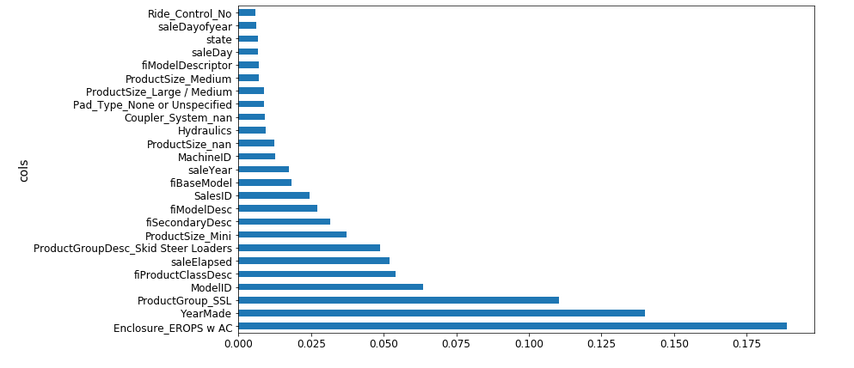
Earlier, YearMade was the most important feature in the dataset, but EROPS w AC has a higher feature importance in the above chart. Curious what this variable is? Don’t worry, we will discuss what EROPS w AC actually represents in the following section.

Removing redundant features

So far, we’ve understood that having a high number of features can affect the performance of the model and also make it difficult to interpret the results. In this section, we will see how we can identify redundant features and remove them from the data.

We will use cluster analysis, more specifically hierarchical clustering, to identify similar variables. In this technique, we look at every object and identify which of them are the closest in terms of features. These variables are then replaced by their midpoint. To understand this better, let us have a look at the cluster plot for our dataset:

from scipy.cluster import hierarchy as hc
corr = np.round(scipy.stats.spearmanr(df_keep).correlation, 4)
corr_condensed = hc.distance.squareform(1-corr)
z = hc.linkage(corr_condensed, method='average')
fig = plt.figure(figsize=(16,10))
dendrogram = hc.dendrogram(z, labels=df_keep.columns,
    orientation='left', leaf_font_size=16)
plt.show()

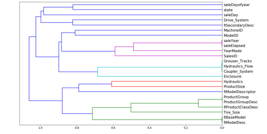
From the above dendrogram plot, we can see that the variables SaleYear and SaleElapsed are very similar to each other and tend to represent the same thing. Similarly, Grouser_Tracks, Hydraulics_Flow, and Coupler_System are highly correlated. The same happens with ProductGroup & ProductGroupDesc and fiBaseModel & fiModelDesc. We will remove each of these features one by one and see how it affects the model performance.

First, we define a function to calculate the Out of Bag (OOB) score (to avoid repeating the same lines of code):

#define function to calculate oob score
def get_oob(df):
  m = RandomForestRegressor(n_estimators=30, min_samples_leaf=5, max_features=0.6, n_jobs=-1, oob_score=True)
  x, _ = split_vals(df, n_trn)
  m.fit(x, y_train)
  return m.oob_score_

For the sake of comparison, below is the original OOB score before dropping any feature:

get_oob(df_keep)
0.89019425494301454

We will now drop one variable at a time and calculate the score:

for c in ('saleYear', 'saleElapsed', 'fiModelDesc', 'fiBaseModel', 'Grouser_Tracks', 'Coupler_System'):
  print(c, get_oob(df_keep.drop(c, axis=1)))

saleYear 0.889037446375
saleElapsed 0.886210803445
fiModelDesc 0.888540591321
fiBaseModel 0.88893958239
Grouser_Tracks 0.890385236272
Coupler_System 0.889601052658

This hasn’t heavily affected the OOB score. Let us now remove one variable from each pair and check the overall score:

to_drop = ['saleYear', 'fiBaseModel', 'Grouser_Tracks']
get_oob(df_keep.drop(to_drop, axis=1))
0.88858458047200739

The score has changed from 0.8901 to 0.8885. We will use these selected features on the complete dataset and see how our model performs:

df_keep.drop(to_drop, axis=1, inplace=True)
X_train, X_valid = split_vals(df_keep, n_trn)
reset_rf_samples()

m = RandomForestRegressor(n_estimators=40, min_samples_leaf=3, max_features=0.5, n_jobs=-1, oob_score=True)
m.fit(X_train, y_train)
print_score(m)

[0.12615142089579687, 0.22781819082173235, 0.96677727309424211, 0.90731173105384466, 0.9084359846323049]

Once these variables are removed from the original dataframe, the model’s score turns out to be 0.907 on the validation set.

Partial Dependence

I’ll introduce another technique here that has the potential to help us understand the data better. This technique is called Partial Dependence and it’s used to find out how features are related to the target variable.

from pdpbox import pdp
from plotnine import *

set_rf_samples(50000)

df_trn2, y_trn, nas = proc_df(df_raw, 'SalePrice', max_n_cat=7)
X_train, X_valid = split_vals(df_trn2, n_trn)
m = RandomForestRegressor(n_estimators=40, min_samples_leaf=3, max_features=0.6, n_jobs=-1)
m.fit(X_train, y_train);

plot_fi(rf_feat_importance(m, df_trn2)[:10]);

Let us compare YearMade and SalePrice. If you create a scatter plot for YearMade and SaleElapsed, you’d notice that some vehicles were created in the year 1000, which is not practically possible.

df_raw.plot('YearMade', 'saleElapsed', 'scatter', alpha=0.01, figsize=(10,8));

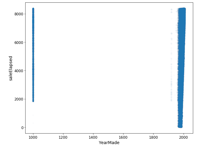
These could be the values which were initially missing and have been replaced with 1,000. To keep things practical, we will focus on values that are greater than 1930 for the YearMade variable and create a plot using the popular ggplot package.

x_all = get_sample(df_raw[df_raw.YearMade>1930], 500)
ggplot(x_all, aes('YearMade', 'SalePrice'))+stat_smooth(se=True, method='loess')

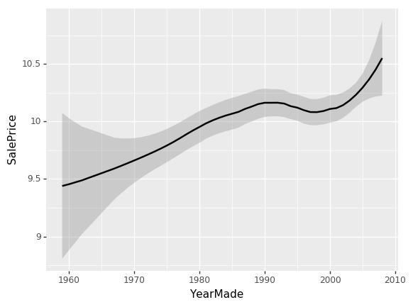
This plot shows that the sale price is higher for more recently made vehicles, except for one drop between 1991 and 1997. There could be various reasons for this drop – recession, customers preferred vehicles of lower price, or some other external factor. To understand this, we will create a plot that shows the relationship between YearMade and SalePrice, given that all other feature values are the same.

x = get_sample(X_train[X_train.YearMade>1930], 500)

def plot_pdp(feat, clusters=None, feat_name=None):
   feat_name = feat_name or feat
   p = pdp.pdp_isolate(m, x, feat)
   return pdp.pdp_plot(p, feat_name, plot_lines=True, cluster=clusters is not None, n_cluster_centers=clusters)

plot_pdp('YearMade')

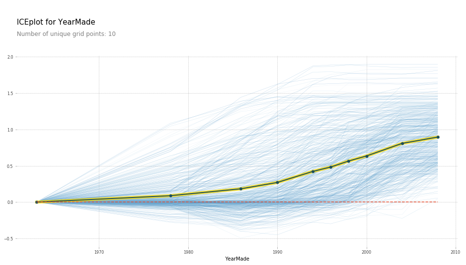
This plot is obtained by fixing the YearMade for each row to 1960, then 1961, and so on. In simple words, we take a set of rows and calculate SalePrice for each row when YearMade is 1960. Then we take the whole set again and calculate SalePrice by setting YearMade to 1962. We repeat this multiple times, which results in the multiple blue lines we see in the above plot. The dark black line represents the average. This confirms our hypothesis that the sale price increases for more recently manufactured vehicles.

Similarly, you can check for other features like SaleElapsed, or YearMade and SaleElpased together. Performing the same step for the categories under Enclosure (since Enclosure_EROPS w AC proved to be one of the most important features), the resulting plot looks like this:

plot_pdp(['Enclosure_EROPS w AC', 'Enclosure_EROPS', 'Enclosure_OROPS'], 5, 'Enclosure')

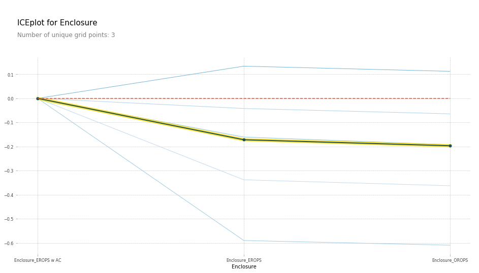
Enclosure_EROPS w AC seems to have a higher sale price as compared to the other two variables (which have almost equal values). So what in the world is EROPS? It’s an enclosed rollover protective structure which can be with or without an AC. And obviously, EROPS with an AC will have a higher sale price.

Tree Interpreter

Tree interpreter in another interesting technique that analyzes each individual row in the dataset. We have seen so far how to interpret a model, and how each feature (and the levels in each categorical feature) affect the model predictions. So we will now use this tree interpreter concept and visualize the predictions for a particular row.

Let’s import the tree interpreter library and evaluate the results for the first row in the validation set.

from treeinterpreter import treeinterpreter as ti
df_train, df_valid = split_vals(df_raw[df_keep.columns], n_trn)
row = X_valid.values[None,0]
row

array([[4364751, 2300944, 665, 172, 1.0, 1999, 3726.0, 3, 3232, 1111, 0, 63, 0, 5, 17, 35, 4, 4, 0, 1, 0, 0,
       0, 0, 0, 0, 0, 0, 0, 0, 12, 0, 0, 0, 0, 0, 3, 0, 0, 0, 2, 19, 29, 3, 2, 1, 0, 0, 0, 0, 0, 2010, 9, 37,
       16, 3, 259, False, False, False, False, False, False, 7912, False, False]], dtype=object)

These are the original values for first row (and it’s every column) in the validation set. Using tree interpreter, we will make predictions for the same using a random forest model. Tree interpreter gives three results – prediction, bias and contribution.

• Predictions are the values predicted by the random forest model
• Bias is the average value of the target variable for the complete dataset
• Contributions are the amount by which the predicted value was changed by each column

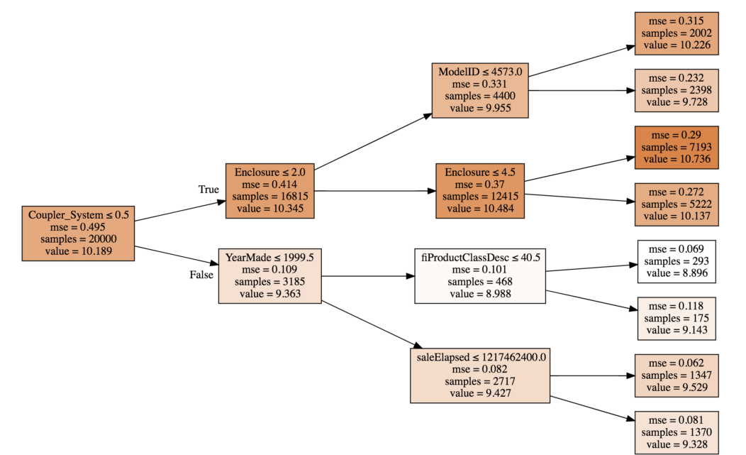
The value of Coupler_System < 0.5 increased the value from 10.189 to 10.345 and enclosure less than 0.2 reduced the value from 10.345 to 9.955, and so on. So the contributions will represent this change in the predicted values. To understand this in a better way, take a look at the table below:

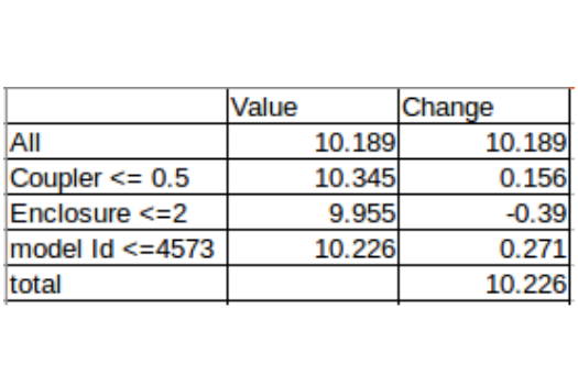
In this table, we have stored the value against each feature and the split point (verify from the image above). The change is the difference between the value before and after the split. These are plotted using a waterfall chart in Excel. The change seen here is for an individual tree. An average of change across all the trees in the random forest is given by contribution in the tree interpreter.

Printing the prediction and bias for the first row in our validation set:

prediction, bias, contributions = ti.predict(m, row)
prediction[0], bias[0]

(9.1909688098736275, 10.10606580677884)

The value of contribution of each feature in the dataset for this first row:

idxs = np.argsort(contributions[0])
[o for o in zip(df_keep.columns[idxs], df_valid.iloc[0][idxs], contributions[0][idxs])]

[('ProductSize', 'Mini', -0.54680742853695008),
('age', 11, -0.12507089451852943),
('fiProductClassDesc',
 'Hydraulic Excavator, Track - 3.0 to 4.0 Metric Tons',
 -0.11143111128570773),
('fiModelDesc', 'KX1212', -0.065155113754146801),
('fiSecondaryDesc', nan, -0.055237427792181749),
('Enclosure', 'EROPS', -0.050467175593900217),
('fiModelDescriptor', nan, -0.042354676935508852),
('saleElapsed', 7912, -0.019642242073500914),
('saleDay', 16, -0.012812993479652724),
('Tire_Size', nan, -0.0029687660942271598),
('SalesID', 4364751, -0.0010443985823001434),
('saleDayofyear', 259, -0.00086540581130196688),
('Drive_System', nan, 0.0015385818526195915),
('Hydraulics', 'Standard', 0.0022411701338458821),
('state', 'Ohio', 0.0037587658190299409),
('ProductGroupDesc', 'Track Excavators', 0.0067688906745931197),
('ProductGroup', 'TEX', 0.014654732626326661),
('MachineID', 2300944, 0.015578052196894499),
('Hydraulics_Flow', nan, 0.028973749866174004),
('ModelID', 665, 0.038307429579276284),
('Coupler_System', nan, 0.052509808150765114),
('YearMade', 1999, 0.071829996446492878)]

Note: If you are watching the video simultaneously with this article, the values may differ. This is because initially the values were sorted based on index which presented incorrect information. This was corrected in the later video and also in the notebook we have been following throughout the lesson.

Introduction to Machine Learning : Lesson 5

You should have a pretty good understanding of the random forest algorithm at this stage. In lesson #5, we will focus on how to identify whether model is generalizing well or not. Jeremy Howard also talks about tree interpreters, contribution, and understanding the same using a waterfall chart (which we have already covered in the previous lesson, so will not elaborate on this further).  The primary focus of the video is on Extrapolation and understanding how we can build a random forest algorithm from scratch.

Extrapolation

A model might not perform well if it’s built on data spanning four years and then used to predict the values for the next one year. In other words, the model does not extrapolate. We have previously seen that there is a significant difference between the training score and validation score, which might be because our validation set consists of a set of recent data points (and the model is using time dependent variables for making predictions).

Also, the validation score is worse than the OOB score which should not be the case, right? A detailed explanation of the OOB score has been given in part 1 of the series. One way of fixing this problem is by attacking it directly – deal with the time dependent variables.

To figure out which variables are time dependent, we will create a random forest model that tries to predict if a particular row is in the validation set or not. Then we will check which variable has the highest contribution in making a successful prediction.

Defining the target variable:

df_ext = df_keep.copy()
df_ext['is_valid'] = 1
df_ext.is_valid[:n_trn] = 0
x, y, nas = proc_df(df_ext, 'is_valid')

m = RandomForestClassifier(n_estimators=40, min_samples_leaf=3, max_features=0.5, n_jobs=-1, oob_score=True)
m.fit(x, y);
m.oob_score_

0.99998753505765037

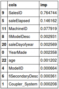
The model is able to separate the train and validation sets with a r-square value 0.99998, and the most important features are SaleID, SaleElapsed, MachineID.

fi = rf_feat_importance(m, x)
fi[:10]

• SaleID is certainly not a random identifier, it should ideally be in an increasing order
• Looks like MachineID has the same trend and is able to separate the train and validation sets
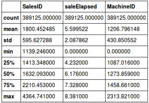
• SaleElapsed  is the number of days from the first date in the dataset. Since our validation set has the most recent values from the complete data, SaleElapsed would be higher in this set. To confirm the hypothesis, here is the distribution of the three variables in train and test:

feats=['SalesID', 'saleElapsed', 'MachineID']
(X_train[feats]/1000).describe()

(X_valid[feats]/1000).describe()

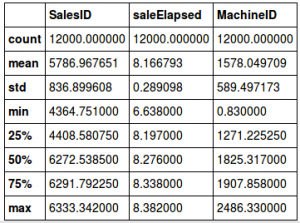
It is evident from the tables above that the mean value of these three variables is significantly different. We will drop these variables, fit the random forest again and check the feature importance:

x.drop(feats, axis=1, inplace=True)
m = RandomForestClassifier(n_estimators=40, min_samples_leaf=3, max_features=0.5, n_jobs=-1, oob_score=True)
m.fit(x, y);
m.oob_score_

0.9789018385789966

fi = rf_feat_importance(m, x)
fi[:10]

Although these variables are obviously time dependent, they can also be important for making the predictions. Before we drop these variables, we need to check how they affect the OOB score. The initial OOB score in a sample is calculated for comparison:

set_rf_samples(50000)
feats=['SalesID', 'saleElapsed', 'MachineID', 'age', 'YearMade', 'saleDayofyear']
X_train, X_valid = split_vals(df_keep, n_trn)
m = RandomForestRegressor(n_estimators=40, min_samples_leaf=3, max_features=0.5, n_jobs=-1, oob_score=True)
m.fit(X_train, y_train)
print_score(m)

[0.21136509778791376, 0.2493668921196425, 0.90909393040946562, 0.88894821098056087, 0.89255408392415925]

Dropping each feature one by one:

for f in feats:

  df_subs = df_keep.drop(f, axis=1)
  X_train, X_valid = split_vals(df_subs, n_trn)
  m = RandomForestRegressor(n_estimators=40, min_samples_leaf=3, max_features=0.5, n_jobs=-1, oob_score=True)
  m.fit(X_train, y_train)
  print(f)
  print_score(m)

SalesID
0.20918653475938534, 0.2459966629213187, 0.9053273181678706, 0.89192968797265737, 0.89245205174299469]

saleElapsed
[0.2194124612957369, 0.2546442621643524, 0.90358104739129086, 0.8841980790762114, 0.88681881032219145]

MachineID
[0.206612984511148, 0.24446409479358033, 0.90312476862123559, 0.89327205732490311, 0.89501553584754967]

age
[0.21317740718919814, 0.2471719147150774, 0.90260198977488226, 0.89089460707372525, 0.89185129799503315]

YearMade
[0.21305398932040326, 0.2534570148977216, 0.90555219348567462, 0.88527538596974953, 0.89158854973045432]

saleDayofyear
[0.21320711524847227, 0.24629839782893828, 0.90881970943169987, 0.89166441133215968, 0.89272793857941679]

Looking at the results, age, MachineID and SaleDayofYear actually improved the score while others did not. So, we will remove the remaining variables and fit the random forest on the complete dataset.

reset_rf_samples()
df_subs = df_keep.drop(['SalesID', 'MachineID', 'saleDayofyear'],axis=1)
X_train, X_valid = split_vals(df_subs, n_trn)
m = RandomForestRegressor(n_estimators=40, min_samples_leaf=3, max_features=0.5, n_jobs=-1, oob_score=True)
m.fit(X_train, y_train)
print_score(m)

[0.1418970082803121, 0.21779153679471935, 0.96040441863389681, 0.91529091848161925, 0.90918594039522138]

After removing the time dependent variables, the validation score (0.915) is now better than the OOB score (0.909). We can now play around with other parameters like n_estimator on max_features. To create the final model, Jeremy increased the number of trees to 160 and here are the results:

m = RandomForestRegressor(n_estimators=160, max_features=0.5, n_jobs=-1, oob_score=True)
%time m.fit(X_train, y_train)
print_score(m)

CPU times: user 6min 3s, sys: 2.75 s, total: 6min 6s
Wall time: 16.7 s
[0.08104912951128229, 0.2109679613161783, 0.9865755186304942, 0.92051576728916762, 0.9143700001430598]

The validation score is 0.92 while the RMSE drops to 0.21. A great improvement indeed!

Random Forest from Scratch

We have learned about how a random forest model actually works, how the features are selected and how predictions are eventually made. In this section, we will create our own random forest model from absolute scratch. Here is the notebook for this section : Random Forest from scratch.

We’ll start with importing the basic libraries:

%load_ext autoreload
%autoreload 2
%matplotlib inline

from fastai.imports import *
from fastai.structured import *
from sklearn.ensemble import RandomForestRegressor, RandomForestClassifier

from IPython.display import display
from sklearn import metrics

We’ll just use two variables to start with. Once we are confident that the model works well with these selected variables, we can use the complete set of features.

PATH = "data/bulldozers/"

df_raw = pd.read_feather('tmp/bulldozers-raw')
df_trn, y_trn, nas = proc_df(df_raw, 'SalePrice')
def split_vals(a,n): return a[:n], a[n:]

n_valid = 12000
n_trn = len(df_trn)-n_valid

X_train, X_valid = split_vals(df_trn, n_trn)
y_train, y_valid = split_vals(y_trn, n_trn)
raw_train, raw_valid = split_vals(df_raw, n_trn)
x_sub = X_train[['YearMade', 'MachineHoursCurrentMeter']]

We have loaded the dataset, split it into train and validation sets, and selected two features – YearMade and MachineHoursCurrentMeter. The first thing to think about while building any model from scratch is – what information do we need? So, for a random forest, we need:

• A set of features – x
• A target variable – y
• Number of trees in the random forest – n_trees
• A variable to define the sample size – sample_sz
• A variable for minimum leaf size – min_leaf
• A random seed for testing

Let’s define a class with the inputs as mentioned above and set the random seed to 42.

class TreeEnsemble():
   def __init__(self, x, y, n_trees, sample_sz, min_leaf=5):
       np.random.seed(42)
       self.x,self.y,self.sample_sz,self.min_leaf = x,y,sample_sz,min_leaf
       self.trees = [self.create_tree() for i in range(n_trees)]

   def create_tree(self):
       rnd_idxs = np.random.permutation(len(self.y))[:self.sample_sz]
       return DecisionTree(self.x.iloc[rnd_idxs], self.y[rnd_idxs], min_leaf=self.min_leaf)
       
   def predict(self, x):
       return np.mean([t.predict(x) for t in self.trees], axis=0)

We have created a function create_trees that will be called as many times as the number assigned to n_trees. The function create_trees generates a randomly shuffled set of rows (of size = sample_sz) and returns DecisionTree. We’ll see DecisionTree in a while, but first let’s figure out how predictions are created and saved.

We learned earlier that in a random forest model, each single tree makes a prediction for each row and the final prediction is calculated by taking the average of all the predictions. So we will create a predict function, where .predict is used on every tree to create a list of predictions and the mean of this list is calculated as our final value.

The final step is to create the DecisionTree. We first select a feature and split point that gives the least error. At present, this code is only for a single decision. We can make this recursive if the code runs successfully.

class DecisionTree():
   def __init__(self, x, y, idxs=None, min_leaf=5):
       if idxs is None: idxs=np.arange(len(y))
       self.x,self.y,self.idxs,self.min_leaf = x,y,idxs,min_leaf
       self.n,self.c = len(idxs), x.shape[1]
       self.val = np.mean(y[idxs])
       self.score = float('inf')
       self.find_varsplit()
       
   # This just does one decision; we'll make it recursive later
   def find_varsplit(self):
       for i in range(self.c): self.find_better_split(i)
           
   # We'll write this later!
   def find_better_split(self, var_idx): pass
   
   @property
   def split_name(self): return self.x.columns[self.var_idx]
   
   @property
   def split_col(self): return self.x.values[self.idxs,self.var_idx]

   @property
   def is_leaf(self): return self.score == float('inf')
   
   def __repr__(self):
       s = f'n: {self.n}; val:{self.val}'
       if not self.is_leaf:
           s += f'; score:{self.score}; split:{self.split}; var:{self.split_name}'
       return s

self.n defines the number of rows used in each tree and self.c is the number of columns. Self.val calculates the mean of predictions for each index. This code is still incomplete and will be continued in the next lesson. Yes, part 3 is coming soon!

Additional Topics

• Reading a large dataset in seconds: The time to load a dataset reduces if we provide the data type of the variables at the time of reading the file itself. Use this dataset which has over a 100 million rows to see this in action.

types = {'id': 'int64',
       'item_nbr': 'int32',
       'store_nbr': 'int8',
       'unit_sales': 'float32',
       'onpromotion': 'object'}
%%time
df_test = pd.read_csv(f'{PATH}test.csv', parse_dates = ['date'], dtype=types, infer_datetime_format=True)

CPU times: user 1min 41s, sys: 5.08s, total: 1min 46s
Wall time: 1min 48s

• Cardinality: This is the number of levels in a categorical variable. For the UsageBand variable, we had three levels – High, Low and Medium. Thus the cardinality is 3.

• Train-validation-test: It is important to have a validation set to check the performance of the model before we use it on the test set. It often happens that we end up overfitting our model on the validation set. And if the validation set is not a true representative of the test set, then the model will fail as well. So the complete data should be split into train, validation and test set, where the test set should only be used at the end (and not during parameter tuning).

• Cross validation: Cross validation set is creating more than one validation set and testing the model on each. The complete data is shuffled and split into groups, taking 5 for instance. Four of these groups are used to train the model and one is used as a validation set. In the next iteration, another four are used for training and one is kept aside for validation. This step will be repeated five times, where each set is used as a validation set once.

End Notes

I consider this one of the most important articles in this ongoing series. I cannot stress enough on how important model interpretability is. In real-life industry scenarios, you will quite often face the situation of having to explain the model’s results to the stakeholder (who is usually a non-technical person).

Your chances of getting the model approved will lie in how well you are able to explain how and why the model is behaving the way it is. Plus it’s always a good idea to always explain any model’s performance to yourself in a way that a layman will understand – this is always a good practice!

Use the comments section below to let me know your thoughts or ask any questions you might have on this article. And as I mentioned, part 3 is coming soon so stay tuned!

Aishwarya Singh

An avid reader and blogger who loves exploring the endless world of data science and artificial intelligence. Fascinated by the limitless applications of ML and AI; eager to learn and discover the depths of data science.