Getting Started with Machine Learning -  Implementing Linear Regression from Scratch

This article was published as a part of the Data Science Blogathon

Introduction

Using the machine learning models in your projects is quite simple considering that we have pre-built modules and libraries like sklearn, but it is important that one knows how the actual algorithm works for a better understanding of the core concept. In this blog, we will be implementing one of the most basic algorithms in machine learning i.e Simple Linear Regression. The topics that will be covered in this blog are as follows:

What is Linear Regression?

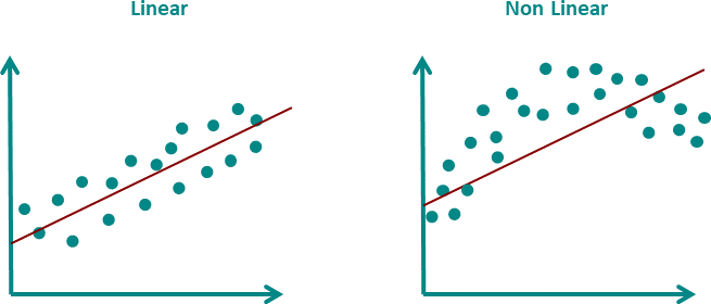
Linear Regression is a supervised Machine Learning algorithm it is also considered to be the most simple type of predictive Machine Learning algorithm. There is some basic assumption that we make for linear regression to work, such as it is important that the relation between the independent and the target variable is linear in nature else our model will end up giving irrelevant results.

Image Link

The word Linear in Linear Regression suggests that the function used for the prediction is a linear function. This function can be represented as shown below:

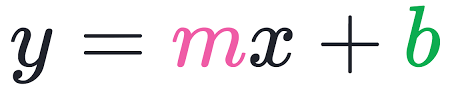
Now, you might be familiar with this equation, in fact, we all have used this equation this is the equation of a straight line. In terms of linear regression, y in this equation stands for the predicted value, x means the independent variable and m & b are the coefficients we need to optimize in order to fit the regression line to our data.

Calculating coefficient of the equation:

To calculate the coefficients we need the formula for Covariance and Variance, so the formula for these are:

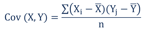
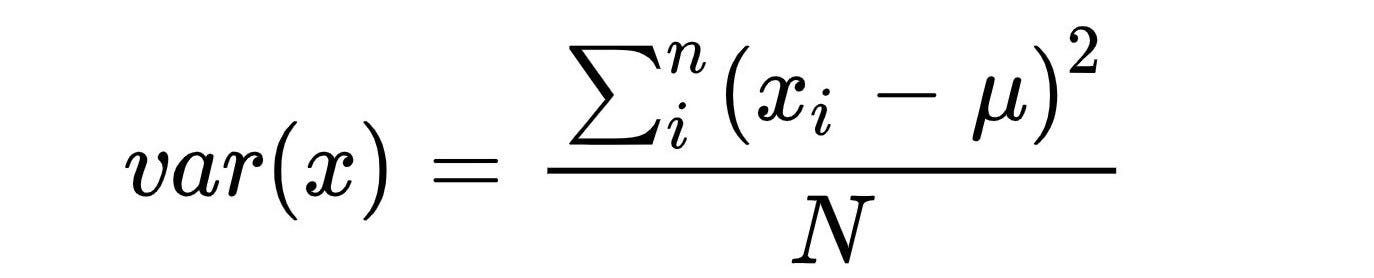
To calculate the coefficient m we will use the formula given below

m = cov(x, y) / var(x)
b = mean(y) — m * mean(x)

How to implement Linear Regression in Python?

Now that we know the formulas for calculating the coefficients of the equation let’s move onto the implementation. To implement this code we will be using standard libraries like Pandas and Numpy and later to visualize our result we will use Matplotlib and Seaborn.

The dataset used in this example is available on my Github repository here. The dataset has 2 columns Parameter 1 and Parameter 2. So, x will be Parameter 1 and y will be Parameter 2. We will first start by writing functions to calculate the Mean, Covariance, and Variance.

# mean 
def get_mean(arr):
    return np.sum(arr)/len(arr)

# variance
def get_variance(arr, mean):
    return np.sum((arr-mean)**2)

# covariance
def get_covariance(arr_x, mean_x, arr_y, mean_y):
    final_arr = (arr_x - mean_x)*(arr_y - mean_y)
    return np.sum(final_arr)

Now, the next step will be to calculate the coefficients and the Linear Regression Function so let’s see the code for those functions.

# Coefficients 
# m = cov(x, y) / var(x)
# b = y - m*x
def get_coefficients(x, y):
    x_mean = get_mean(x)
    y_mean = get_mean(y)
    m = get_covariance(x, x_mean, y, y_mean)/get_variance(x, x_mean)
    b = y_mean - x_mean*m
    return m, b

# Linear Regression 
# Train and Test
# Train Split 80 % Test Split 20 %
def linear_regression(x_train, y_train, x_test, y_test):
    prediction = []
    m, b = get_coefficients(x_train, y_train)
    for x in x_test:
        y = m*x + b
        prediction.append(y)
    
    r2 = r2_score(prediction, y_test)
    mse = mean_squared_error(prediction, y_test)
    print("The R2 score of the model is: ", r2)
    print("The MSE score of the model is: ", mse)
    return prediction
prediction = linear_regression(x[:80], y[:80], x[80:], y[80:])

Now that we have all the functions ready for implementing the regression, the only thing that remains is the visualization, so now we will write the code to visualize the regression line.

How to visualize the regression line?

To visualize the regression line we will use the matplotlib and seaborn libraries. The points will be plotted using the scatterplot and the regression line will be plotted using the lineplot functions. Seaborn also offers a separate plot for regression called the regplot (regression plot) but here we will be using the scatter and lineplot for visualizing the line.

def plot_reg_line(x, y):
    # Calculate predictions for x ranging from 1 to 100
    prediction = []
    m, c = get_coefficients(x, y)
    for x0 in range(1,100):
        yhat = m*x0 + c
        prediction.append(yhat)
    
    # Scatter plot without regression line
    fig = plt.figure(figsize=(20,7))
    plt.subplot(1,2,1)
    sns.scatterplot(x=x, y=y)
    plt.xlabel('X')
    plt.ylabel('Y')
    plt.title('Scatter Plot between X and Y')
    
    # Scatter plot with regression line
    plt.subplot(1,2,2)
    sns.scatterplot(x=x, y=y, color = 'blue')
    sns.lineplot(x = [i for i in range(1, 100)], y = prediction, color='red')
    plt.xlabel('X')
    plt.ylabel('Y')
    plt.title('Regression Plot')
    plt.show()

The above code is for understanding the way our visualization works but for regular use you need not write the above code you can simply use the regplot from seaborn, regplot is basically the combination of the scatter plot and the line plot, the code for regplot is as shown below.

# Regression plot
sns.regplot(x, y)
plt.xlabel('X')
plt.ylabel('Y')
plt.title("Regression Plot")
plt.show()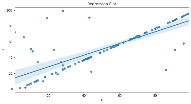

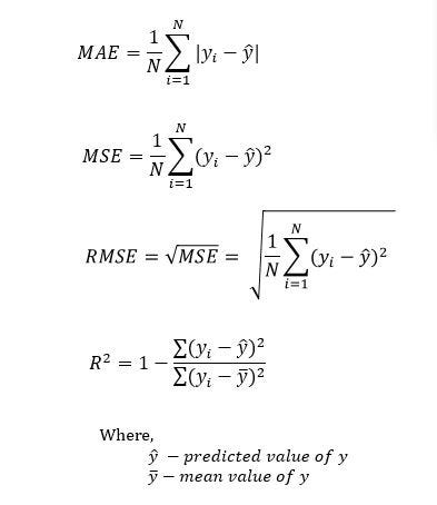
Which metrics to use for model evaluation?

For evaluation of a regression model we generally use the

1. r2_score
2. mean_squared_error
3. root_mean_squared_error
4. mean_absolute_error

You can learn about these metrics here. In this blog, we have made use of 2 metrics from the 3 listed above. The r2_score and mean_squared_error. The r2_score ranges from 0 to 1 where 1 signifies absolute precision and 0 signify poor performance, the mse or the mean squared error is basically the summation of all the squared errors and lesser the mse value better our model is.

Results and Conclusion:

So now we will combine all the codes we have written above and look at the results we obtain, we will make use of both, the algorithm coded by us as well as the built-in library sklearn. If results by both the methods are the same it means we have successfully coded the algorithm.

Let’s first look at our algorithm:

# Import necessary Libraries
import numpy as np
import pandas as pd
import matplotlib.pyplot as plt
import seaborn as sns
from sklearn.metrics import r2_score, mean_squared_error

# Read Data
df = pd.read_csv('SampleData.csv')
x = df['Parameter 1'].values
y = df['Parameter 2'].values

# mean
def get_mean(arr):
    return np.sum(arr)/len(arr)

# variance
def get_variance(arr, mean):
    return np.sum((arr-mean)**2)

# covariance
def get_covariance(arr_x, mean_x, arr_y, mean_y):
    final_arr = (arr_x - mean_x)*(arr_y - mean_y)
    return np.sum(final_arr)

# find coeff
def get_coefficients(x, y):
    x_mean = get_mean(x)
    y_mean = get_mean(y)
    m = get_covariance(x, x_mean, y, y_mean)/get_variance(x, x_mean)
    c = y_mean - x_mean*m
    return m, c

# Regression Function
def linear_regression(x_train, y_train, x_test, y_test):
    prediction = []
    m, c = get_coefficients(x_train, y_train)
    for x in x_test:
        y = m*x + c
        prediction.append(y)
    
    r2 = r2_score(prediction, y_test)
    mse = mean_squared_error(prediction, y_test)
    print("The R2 score of the model is: ", r2)
    print("The MSE score of the model is: ", mse)
    return prediction

# There are 100 sample out of which 80 are for training and 20 are for testing
linear_regression(x[:80], y[:80], x[80:], y[80:])

# Visualize
def plot_reg_line(x, y):
    prediction = []
    m, c = get_coefficients(x, y)
    for x0 in range(1,100):
        yhat = m*x0 + c
        prediction.append(yhat)
    
    fig = plt.figure(figsize=(20,7))
    plt.subplot(1,2,1)
    sns.scatterplot(x=x, y=y)
    plt.xlabel('X')
    plt.ylabel('Y')
    plt.title('Scatter Plot between X and Y')
    
    plt.subplot(1,2,2)
    sns.scatterplot(x=x, y=y, color = 'blue')
    sns.lineplot(x = [i for i in range(1, 100)], y = prediction, color='red')
    plt.xlabel('X')
    plt.ylabel('Y')
    plt.title('Regression Plot')
    plt.show()
    
plot_reg_line(x, y)

And the output generated by our algorithm is shown the figure below, the red line shows the regression line.

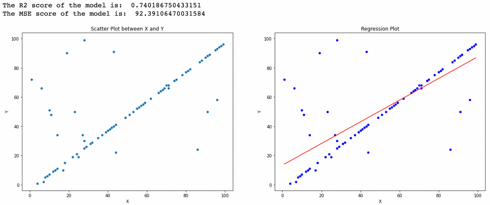
Now let’s see the built-in Linear Regression function:

import numpy as np
import pandas as pd
import matplotlib.pyplot as plt
import seaborn as sns
from sklearn.metrics import r2_score, mean_squared_error
from sklearn.linear_model import LinearRegression

df = pd.read_csv('SampleData.csv')
x = df['Parameter 1'].values
y = df['Parameter 2'].values

reg = LinearRegression()
reg.fit(x[:80].reshape(-1, 1), y[:80])
prediction = reg.predict(x[80:].reshape(-1, 1))
r2 = r2_score(prediction, y[80:])
mse = mean_squared_error(prediction, y[80:])
print("The R2 score of the model is: ", r2)
print("The MSE score of the model is: ", mse)

prediction = reg.predict(np.array([i for i in range(1, 100)]).reshape(-1, 1))

fig = plt.figure(figsize=(20,7))
plt.subplot(1,2,1)
sns.scatterplot(x=x, y=y)
plt.xlabel('X')
plt.ylabel('Y')
plt.title('Scatter Plot between X and Y')

plt.subplot(1,2,2)
sns.scatterplot(x=x, y=y, color = 'green')
sns.lineplot(x = [i for i in range(1, 100)], y = prediction, color='red')
plt.xlabel('X')
plt.ylabel('Y')
plt.title('Regression Plot')
plt.show()

The output of the code above:

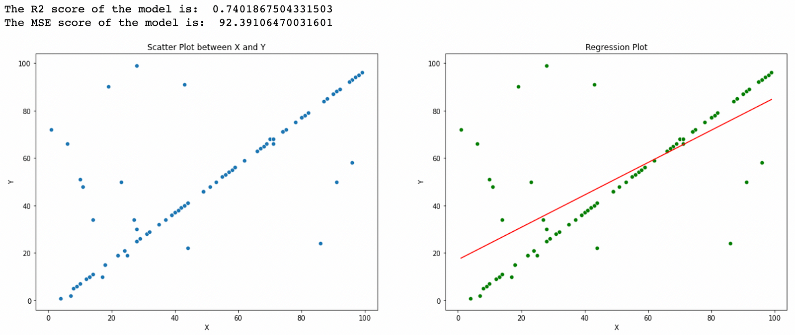
We can clearly see from both the outputs that we have obtained the exact same result from both the algorithms i.e the one we coded and the one in sklearn, so that was all about writing your own code for implementing Linear Regression in python. If you enjoyed reading the blog do share it with your friends. If you have any suggestions or doubts you can comment them down below. in the future blogs, I will try to cover the implementations of other ML algorithms like KNN, Decision Tree, etc. Happy Learning!

Frequently Asked Questions

Connect with me on LinkedIn

Email: [email protected]

Check out my previous articles here.

The media shown in this article are not owned by Analytics Vidhya and are used at the Author’s discretion