Introduction
Statistics is one of the key fundamental skills required for data science. Any expert in data science would surely recommend learning / upskilling yourself in statistics.
However, if you go out and look for resources on statistics, you will see that a lot of them tend to focus on the mathematics. They will focus on derivation of formulas rather than simplifying the concept. I believe, statistics can be understood in very simple and practical manner. That is why I have created this guide.
In this guide, I will take you through Inferential Statistics, which is one of the most important concepts in statistics for data science. I will take you through all the related concepts of Inferential Statistics and their practical applications.
This guide would act as a comprehensive resource to learn Inferential Statistics. So, go through the guide, section by section. Work through the examples and develop your statistics skills for data science.
Read on!
Table of Contents
- Why we need Inferential Statistics?
- Pre-requisites
- Sampling Distribution and Central Limit Theorem
- Hypothesis Testing
- Types of Error in Hypothesis Testing
- T-tests
- Different types of t-test
- ANOVA
- Chi-Square Goodness of Fit
- Regression and ANOVA
- Coefficient of Determination (R-Squared)
1. Why do we need Inferential Statistics?
Suppose, you want to know the average salary of Data Science professionals in India. Which of the following methods can be used to calculate it?
- Meet every Data Science professional in India. Note down their salaries and then calculate the total average?
- Or hand pick a number of professionals in a city like Gurgaon. Note down their salaries and use it to calculate the Indian average.
Well, the first method is not impossible but it would require an enormous amount of resources and time. But today, companies want to make decisions swiftly and in a cost-effective way, so the first method doesn’t stand a chance.
On the other hand, second method seems feasible. But, there is a caveat. What if the population of Gurgaon is not reflective of the entire population of India? There are then good chances of you making a very wrong estimate of the salary of Indian Data Science professionals.
Now, what method can be used to estimate the average salary of all data scientists across India?
Enter Inferential Statistics
In simple language, Inferential Statistics is used to draw inferences beyond the immediate data available.
With the help of inferential statistics, we can answer the following questions:
- Making inferences about the population from the sample.
- Concluding whether a sample is significantly different from the population. For example, let’s say you collected the salary details of Data Science professionals in Bangalore. And you observed that the average salary of Bangalore’s data scientists is more than the average salary across India. Now, we can conclude if the difference is statistically significant.
- If adding or removing a feature from a model will really help to improve the model.
- If one model is significantly better than the other?
- Hypothesis testing in general.
I am sure by now you must have got a gist of why inferential statistics is important. I will take you through the various techniques & concepts involved in Inferential statistics. But first, let’s discuss what are the prerequisites for understanding Inferential Statistics.
2. Pre-Requisites
To begin with Inferential Statistics, one must have a good grasp over the following concepts:
- Probability
- Basic knowledge of Probability Distributions
- Descriptive Statistics
If you are not comfortable with either of the three concepts mentioned above, you must go through them before proceeding further.
Throughout the entire article, I will be using a few terminologies quite often. So, here is a brief description of them:
- Statistic – A Single measure of some attribute of a sample. For eg: Mean/Median/Mode of a sample of Data Scientists in Bangalore.
- Population Statistic – The statistic of the entire population in context. For eg: Population mean for the salary of the entire population of Data Scientists across India.
- Sample Statistic – The statistic of a group taken from a population. For eg: Mean of salaries of all Data Scientists in Bangalore.
- Standard Deviation – It is the amount of variation in the population data. It is given by σ.
- Standard Error – It is the amount of variation in the sample data. It is related to Standard Deviation as σ/√n, where, n is the sample size.
3. Sampling Distribution and Central Limit Theorem
Suppose, you note down the salary of any 100 random Data Science professionals in Gurgaon, calculate the mean and repeat the procedure for say like 200 times (arbitrarily).
When you plot a frequency graph of these 200 means, you are likely to get a curve similar to the one below.
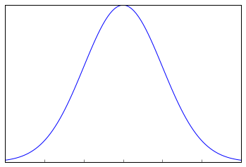
This looks very much similar to the normal curve that you studied in the Descriptive Statistics. This is called Sampling Distribution or the graph obtained by plotting sample means. Let us look at a more formal description of a Sampling Distribution.
A Sampling Distribution is a probability distribution of a statistic obtained through a large number of samples drawn from a specific population.
A Sampling Distribution behaves much like a normal curve and has some interesting properties like :
- The shape of the Sampling Distribution does not reveal anything about the shape of the population. For example, for the above Sampling Distribution, the population distribution may look like the below graph.
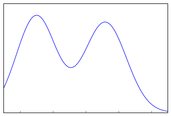
Population Distribution
- Sampling Distribution helps to estimate the population statistic.
But how ?
This will be explained using a very important theorem in statistics – The Central Limit Theorem.
3.1 Central Limit Theorem
It states that when plotting a sampling distribution of means, the mean of sample means will be equal to the population mean. And the sampling distribution will approach a normal distribution with variance equal to σ/√n where σ is the standard deviation of population and n is the sample size.
Points to note:
- Central Limit Theorem holds true irrespective of the type of distribution of the population.
- Now, we have a way to estimate the population mean by just making repeated observations of samples of a fixed size.
- Greater the sample size, lower the standard error and greater the accuracy in determining the population mean from the sample mean.
This seemed too technical isn’t it? Let’s break this down to understand this point by point.
- This means – No matter the shape of the population distribution, be it bi-modal, right skewed etc. The shape of the Sampling Distribution will remain the same (remember the normal curve- bell shaped). This gives us a mathematical advantage to estimate the population statistic – no matter the shape of the population.
- The number of samples have to be sufficient (generally more than 50) to satisfactorily achieve a normal curve distribution. Also, care has to be taken to keep the sample size fixed since any change in sample size will change the shape of the sampling distribution and it will no longer be bell shaped.
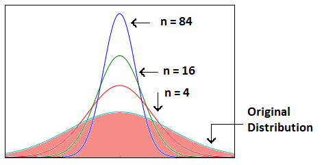
- As we increase the sample size, the sampling distribution squeezes from both sides giving us a better estimate of the population statistic since it lies somewhere in the middle of the sampling distribution (generally). The below image will help you visualize the effect of sample size on the shape of distribution.
Now, since we have collected the samples and plotted their means, it is important to know where the population mean lies with respect to a particular sample mean and how confident can we be about it. This brings us to our next topic – Confidence Interval.
3.2 Confidence Interval
The confidence interval is a type of interval estimate from the sampling distribution which gives a range of values in which the population statistic may lie. Let us understand this with the help of an example.
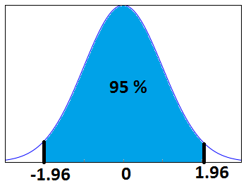
We know that 95% of the values lie within 2 (1.96 to be more accurate) standard deviation of a normal distribution curve. So, for the above curve, the blue shaded portion represents the confidence interval for a sample mean of 0.
Formally, Confidence Interval is defined as,
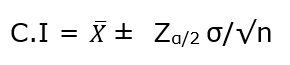
whereas, ![]() = the sample mean
= the sample mean
![]() = Z value for desired confidence level α
= Z value for desired confidence level α
σ = the population standard deviation
For an alpha value of 0.95 i.e 95% confidence interval, z=1.96.
Now there is one more term which you should be familiar with, Margin of Error. It is given as {(z.σ)/√n} and defined as the sampling error by the surveyor or the person who collected the samples. That means, if a sample mean lies in the margin of error range then, it might be possible that its actual value is equal to the population mean and the difference is occurring by chance. Anything outside margin of error is considered statistically significant.
And it is easy to infer that the error can be both positive and negative side. The whole margin of error on both sides of the sample statistic constitutes the Confidence Interval. Numerically, C.I is twice of Margin of Error.
The below image will help you better visualize Margin of Error and Confidence Interval.
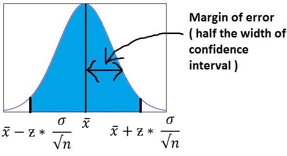
The shaded portion on horizontal axis represents the Confidence Interval and half of it is Margin of Error which can be in either direction of x (bar).
Interesting points to note about Confidence Intervals:
- Confidence Intervals can be built with difference degrees of confidence suitable to a user’s needs like 70 %, 90% etc.
- Greater the sample size, smaller the Confidence Interval, i.e more accurate determination of population mean from the sample means.
- There are different confidence intervals for different sample means. For example, a sample mean of 40 will have a difference confidence interval from a sample mean of 45.
- By 95% Confidence Interval, we do not mean that – The probability of a population mean to lie in an interval is 95%. Instead, 95% C.I means that 95% of the Interval estimates will contain the population statistic.
Many people do not have right knowledge about confidence interval and often interpret it incorrectly. So, I would like you to take your time visualizing the 4th argument and let it sink in.
3.3 Practical example
Calculate the 95% confidence interval for a sample mean of 40 and sample standard deviation of 40 with sample size equal to 100.
Solution:
We know, z-value for 95% C.I is 1.96. Hence, Confidence Interval (C.I) is calculated as:
C.I= [{x(bar) – (z*s/√n)},{x(bar) – (z*s/√n)}]
C.I = [{40-(1.96*40/10},{ 40+(1.96*40/10)}]
C.I = [32.16, 47.84]
4. Hypothesis Testing
Before I get into the theoretical explanation, let us understand Hypothesis Testing by using a simple example.
Example: Class 8th has a mean score of 40 marks out of 100. The principal of the school decided that extra classes are necessary in order to improve the performance of the class. The class scored an average of 45 marks out of 100 after taking extra classes. Can we be sure whether the increase in marks is a result of extra classes or is it just random?
Hypothesis testing lets us identify that. It lets a sample statistic to be checked against a population statistic or statistic of another sample to study any intervention etc. Extra classes being the intervention in the above example.
Hypothesis testing is defined in two terms – Null Hypothesis and Alternate Hypothesis.
- Null Hypothesis being the sample statistic to be equal to the population statistic. For eg: The Null Hypothesis for the above example would be that the average marks after extra class are same as that before the classes.
- Alternate Hypothesis for this example would be that the marks after extra class are significantly different from that before the class.
Hypothesis Testing is done on different levels of confidence and makes use of z-score to calculate the probability. So for a 95% Confidence Interval, anything above the z-threshold for 95% would reject the null hypothesis.
Points to be noted:
- We cannot accept the Null hypothesis, only reject it or fail to reject it.
- As a practical tip, Null hypothesis is generally kept which we want to disprove. For eg: You want to prove that students performed better after taking extra classes on their exam. The Null Hypothesis, in this case, would be that the marks obtained after the classes are same as before the classes.
5. Types of Errors in Hypothesis Testing
Now we have defined a basic Hypothesis Testing framework. It is important to look into some of the mistakes that are committed while performing Hypothesis Testing and try to classify those mistakes if possible.
Now, look at the Null Hypothesis definition above. What we notice at the first look is that it is a statement subjective to the tester like you and me and not a fact. That means there is a possibility that the Null Hypothesis can be true or false and we may end up committing some mistakes on the same lines.
There are two types of errors that are generally encountered while conducting Hypothesis Testing.
- Type I error: Look at the following scenario – A male human tested positive for being pregnant. Is it even possible? This surely looks like a case of False Positive. More formally, it is defined as the incorrect rejection of a True Null Hypothesis. The Null Hypothesis, in this case, would be – Male Human is not pregnant.
- Type II error: Look at another scenario where our Null Hypothesis is – A male human is pregnant and the test supports the Null Hypothesis. This looks like a case of False Negative. More formally it is defined as the acceptance of a false Null Hypothesis.
The below image will summarize the types of error :

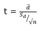
6. T-tests
T-tests are very much similar to the z-scores, the only difference being that instead of the Population Standard Deviation, we now use the Sample Standard Deviation. The rest is same as before, calculating probabilities on basis of t-values.
The Sample Standard Deviation is given as:
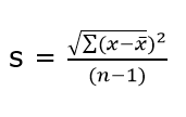
where n-1 is the Bessel’s correction for estimating the population parameter.
Another difference between z-scores and t-values are that t-values are dependent on Degree of Freedom of a sample. Let us define what degree of freedom is for a sample.
The Degree of Freedom – It is the number of variables that have the choice of having more than one arbitrary value. For example, in a sample of size 10 with mean 10, 9 values can be arbitrary but the 1oth value is forced by the sample mean.
Points to note about the t-tests:
- Greater the difference between the sample mean and the population mean, greater the chance of rejecting the Null Hypothesis. Why? (We discussed this above.)
- Greater the sample size, greater the chance of rejection of Null Hypothesis.
7. Different types of t-tests
7.1 1-sample t-test
This is the same test as we described above. This test is used to:
- Determine whether the mean of a group differs from the specified value.
- Calculate a range of values that are likely to include the population mean.
For eg: A pizza delivery manager may perform a 1-sample t-test whether their delivery time is significantly different from that of the advertised time of 30 minutes by their competitors.
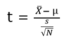
where, X(bar) = sample mean
μ = population mean
s = sample standard deviation
N = sample size
7.2 Paired t-test
Paired t-test is performed to check whether there is a difference in mean after a treatment on a sample in comparison to before. It checks whether the Null hypothesis: The difference between the means is Zero, can be rejected or not.
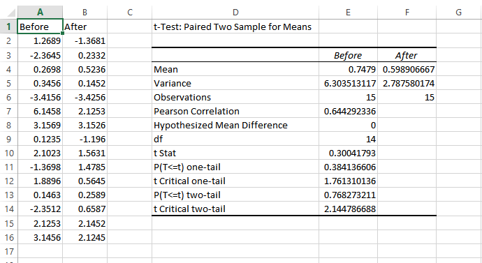
The above example suggests that the Null Hypothesis should not be rejected and that there is no significant difference in means before and after the intervention since p-value is not less than the alpha value (o.o5) and t stat is not less than t-critical. The excel sheet for the above exercise is available here.
where, d (bar) = mean of the case wise difference between before and after,
![]() = standard deviation of the difference
= standard deviation of the difference
n = sample size.
7.3 2-sample t-test
This test is used to determine:
- Determine whether the means of two independent groups differ.
- Calculate a range of values that is likely to include the difference between the population means.
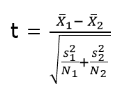
The above formula represents the 2 sample t-test and can be used in situations like to check whether two machines are producing the same output. The points to be noted for this test are:
- The groups to be tested should be independent.
- The groups’ distribution should not be highly skewed.
where, X1 (bar) = mean of the first group
![]() = represents 1st group sample standard deviation
= represents 1st group sample standard deviation
![]() = represents the 1st group sample size.
= represents the 1st group sample size.
7.4 Practical example
We will understand how to identify which t-test to be used and then proceed on to solve it. The other t-tests will follow the same argument.
Example: A population has mean weight of 68 kg. A random sample of size 25 has a mean weight of 70 with standard deviation =4. Identify whether this sample is representative of the population?
Step 0: Identifying the type of t-test
Number of samples in question = 1
Number of times the sample is in study = 1
Any intervention on sample = No
Recommended t-test = 1- sample t-test.
Had there been 2 samples, we would have opted for 2-sample t-test and if there would have been 2 observations on the same sample, we would have opted for paired t-test.`
Step 1: State the Null and Alternate Hypothesis
Null Hypothesis: The sample mean and population mean are same.
Alternate Hypothesis: The sample mean and population mean are different.
Step 2: Calculate the appropriate test statistic
df = 25-1 =24
t= (70-68)/(4/√25) = 2.5
Now, for a 95% confidence level, t-critical (two-tail) for rejecting Null Hypothesis for 24 d.f is 2.06 . Hence, we can reject the Null Hypothesis and conclude that the two means are different.
You can use the t-test calculator here.
8. ANOVA
ANOVA (Analysis of Variance) is used to check if at least one of two or more groups have statistically different means. Now, the question arises – Why do we need another test for checking the difference of means between independent groups? Why can we not use multiple t-tests to check for the difference in means?
The answer is simple. Multiple t-tests will have a compound effect on the error rate of the result. Performing t-test thrice will give an error rate of ~15% which is too high, whereas ANOVA keeps it at 5% for a 95% confidence interval.
To perform an ANOVA, you must have a continuous response variable and at least one categorical factor with two or more levels. ANOVA requires data from approximately normally distributed populations with equal variances between factor levels. However, ANOVA procedures work quite well even if the normality assumption has been violated unless one or more of the distributions are highly skewed or if the variances are quite different.
ANOVA is measured using a statistic known as F-Ratio. It is defined as the ratio of Mean Square (between groups) to the Mean Square (within group).
Mean Square (between groups) = Sum of Squares (between groups) / degree of freedom (between groups)
Mean Square (within group) = Sum of Squares (within group) / degree of freedom (within group)

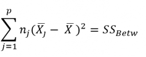
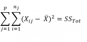
Here, p = represents the number of groups
n = represents the number of observations in a group
![]() = represents the mean of a particular group
= represents the mean of a particular group
X (bar) = represents the mean of all the observations
Now, let us understand the degree of freedom for within group and between groups respectively.
Between groups : If there are k groups in ANOVA model, then k-1 will be independent. Hence, k-1 degree of freedom.
Within groups : If N represents the total observations in ANOVA (∑n over all groups) and k are the number of groups then, there will be k fixed points. Hence, N-k degree of freedom.
8.1 Steps to perform ANOVA
- Hypothesis Generation
- Null Hypothesis : Means of all the groups are same
- Alternate Hypothesis : Mean of at least one group is different
- Calculate within group and between groups variability
- Calculate F-Ratio
- Calculate probability using F-table
- Reject/fail to Reject Null Hypothesis
There are various other forms of ANOVA too like Two-way ANOVA, MANOVA, ANCOVA etc. but One-Way ANOVA suffices the requirements of this course.
Practical applications of ANOVA in modeling are:
- Identifying whether a categorical variable is relevant to a continuous variable.
- Identifying whether a treatment was effective to the model or not.
8.2 Practical Example
Suppose there are 3 chocolates in town and their sweetness is quantified by some metric (S). Data is collected on the three chocolates. You are given the task to identify whether the mean sweetness of the 3 chocolates are different. The data is given as below:
Type A Type B Type C
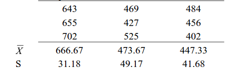
Here, first we have calculated the sample mean and sample standard deviation for you.
Now we will proceed step-wise to calculate the F-Ratio (ANOVA statistic).
Step 1: Stating the Null and Alternate Hypothesis
Null Hypothesis: Mean sweetness of the three chocolates are same.
Alternate Hypothesis: Mean sweetness of at least one of the chocolates is different.
Step 2: Calculating the appropriate ANOVA statistic
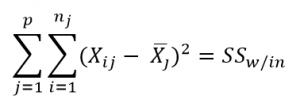
In this part, we will be calculating SS(B), SS(W), SS(T) and then move on to calculate MS(B) and MS(W). The thing to note is that,
Total Sum of Squares [SS(t)] = Between Sum of Squares [SS(B)] + Within Sum of Squares [SS(W)].
So, we need to calculate any two of the three parameters using the data table and formulas given above.
As, per the formula above, we need one more statistic i.e Grand Mean denoted by X(bar) in the formula above.
X bar = (643+655+702+469+427+525+484+456+402)/9 = 529.22
SS(B)=[3*(666.67-529.22)^2]+ [3*(473.67-529.22)^2]+[3*(447.33-529.22)^2] = 86049.55
SS (W) = [(643-666.67)^2+(655-666.67)^2+(702-666.67)^2] + [(469-473.67)^2+(427-473.67)^2+(525-473.67)^2] + [(484-447.33)^2+(456-447.33)^2+(402-447.33)^2]= 10254
MS(B) = SS(B) / df(B) = 86049.55 / (3-1) = 43024.78
MS(W) = SS(W) / df(W) = 10254/(9-3) = 1709
F-Ratio = MS(B) / MS(W) = 25.17 .
Now, for a 95 % confidence level, F-critical to reject Null Hypothesis for degrees of freedom(2,6) is 5.14 but we have 25.17 as our F-Ratio.
So, we can confidently reject the Null Hypothesis and come to a conclusion that at least one of the chocolate has a mean sweetness different from the others.
You can use the F-calculator here.
Note: ANOVA only lets us know the means for different groups are same or not. It doesn’t help us identify which mean is different.To know which group mean is different, we can use another test know as Least Significant Difference Test.
9. Chi-square Goodness of Fit Test
Sometimes, the variable under study is not a continuous variable but a categorical variable. Chi-square test is used when we have one single categorical variable from the population.
Let us understand this with help of an example. Suppose a company that manufactures chocolates, states that they manufacture 30% dairy milk, 60% temptation and 10% kit-kat. Now suppose a random sample of 100 chocolates has 50 dairy milk, 45 temptation and 5 kitkats. Does this support the claim made by the company?
Let us state our Hypothesis first.
Null Hypothesis: The claims are True
Alternate Hypothesis: The claims are False.
Chi-Square Test is given by:
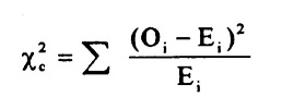
where, ![]() = sample or observed values
= sample or observed values
![]() = population values
= population values
The summation is taken over all the levels of a categorical variable.
![]() = [n *
= [n * ![]() ] Expected value of a level (i) is equal to the product of sample size and percentage of it in the population.
] Expected value of a level (i) is equal to the product of sample size and percentage of it in the population.
Let us now calculate the Expected values of all the levels.
E (dairy milk)= 100 * 30% = 30
E (temptation) = 100 * 60% =60
E (kitkat) = 100 * 10% = 10
Calculating chi-square = [(50-30)^2/30+(45-60)^2/60+(5-10)^2/10] =19.58
Now, checking for p (chi-square >19.58) using chi-square calculator, we get p=0.0001. This is significantly lower than the alpha(0.05).
So we reject the Null Hypothesis.
10. Regression and ANOVA
If you have studied some basic Machine Learning Algorithms, the first algorithm that you must have studied is Regression. If we recall those lessons of Regression, what we generally do is calculate the weights for features present in the model to better predict the output variable. But finding the right set of feature weights or features for that matter is not always possible.
It is highly likely that that the existing features in the model are not fit for explaining the trend in dependent variable or the feature weights calculated fail at explaining the trend in dependent variable. What is important is knowing the degree to which our model is successful in explaining the trend (variance) in dependent variable.
Enter ANOVA.
With the help of ANOVA techniques, we can analyse a model performance very much like we analyse samples for being statistically different or not.
But with regression things are not easy. We do not have mean of any kind to compare or sample as such but we can find good alternatives in our regression model which can substitute for mean and sample.
Sample in case of regression is a regression model itself with pre-defined features and feature weights whereas mean is replaced by variance(of both dependent and independent variables).
Through our ANOVA test we would like to know the amount of variance explained by the Independent variables in Dependent Variable VS the amount of variance that was left unexplained.
It is intuitive to see that larger the unexplained variance(trend) of the dependent variable smaller will be the ratio and less effective is our regression model. On the other hand, if we have a large explained variance then it is easy to see that our regression model was successful in explaining the variance in the dependent variable and more effective is our model. The ratio of Explained Variance uand Unexplained Variance is called F-Ratio.
Let us now define these explained and unexplained variances to find the effectiveness of our model.
1. Regression (Explained) Sum of Squares – It is defined as the amount of variation explained by the Regression model in the dependent variable.
Mathematically, it is calculated as:

where, ![]() [hat] = predicted value and
[hat] = predicted value and
y(bar) = mean of the actual y values.
Interpreting Regression sum of squares –
If our model is a good model for the problem at hand then it would produce an output which has distribution as same to the actual dependent variable. i.e it would be able to capture the inherent variation in the dependent variable.
2. Residual Sum of Squares – It is defined as the amount of variation independent variable which is not explained by the Regression model.
Mathematically, it is calculated as:

where, ![]() = actual ‘y ‘ value
= actual ‘y ‘ value
f(x) = predicted value
Interpretation of Residual Sum of Squares –
It can be interpreted as the amount by which the predicted values deviated from the actual values. Large deviation would indicate that the model failed at predicting the correct values for the dependent variable.
Let us now work out F-ratio step by step. We will be making using of the Hypothesis Testing framework described above to test the significance of the model.
While calculating the F-Ratio care has to be taken to incorporate the effect of degree of freedom. Mathematically, F-Ratio is the ratio of [Regression Sum of Squares/df(regression)] and [Residual Sum of Squares/df(residual)].
We will be understanding the entire concept using an example and this excel sheet.
Step 0: State the Null and Alternate Hypothesis
Null Hypothesis: The model is unable to explain the variance in the dependent variable (Y).
Alternate Hypothesis: The model is able to explain the variance in dependent variable (Y)
Step 1:
Calculate the regression equation for X and Y using Excel’s in-built tool.
Step 2:
Predict the values of y for each row of data.
Step 3:
Calculate y(mean) – mean of the actual y values which in this case turns out to be 0.4293548387.
Step 4:
Calculate the Regression Sum of Squares using the above-mentioned formula. It turned out to be 2.1103632473
The Degree of freedom for regression equation is 1, since we have only 1 independent variable.
Step 5:
Calculate the Residual Sum of Squares using the above-mentioned formula. It turned out to be 0.672210946.
Degree of Freedom for residual = Total degree of freedom – Degree of freedom(regression)
=(62-1) – 1 = 60
Step 6:
F-Ratio = (2.1103632473/1)/(0.672210946/60) = 188.366
Now, for 95% confidence, F-critical to reject Null Hypothesis for 1,60 degrees of freedom in 4. But we have F-ratio as 188, so we can safely reject the Null Hypothesis and conclude that model explains variation to a large extent.
11. Coefficient of Determination (R-Square)
It is defined as the ratio of the amount of variance explained by the regression model to the total variation in the data. It represents the strength of correlation between two variables.
We already calculated the Regression SS and Residual SS. Total SS is the sum of Regression SS and Residual SS.
Total SS = 2.1103632473+ 0.672210946 = 2.78257419
Co-efficient of Determination = 2.1103632473/2.78257419 = 0.7588
12. Correlation Coefficient
This is another useful statistic which is used to determine the correlation between two variables. It is simply the square root of coefficient of Determination and ranges from -1 to 1 where 0 represents no correlation and 1 represents positive strong correlation while -1 represents negative strong correlation.
End Notes
So, this guide comes to an end with explaining all the theory along with practical implementations of various Inferential Statistics concepts. This guide has been created with a Hypothesis Testing framework and I hope this would be one stop solution for a quick Inferential Statistics guide.
If you have any doubts or questions, feel free to drop your comments below. And in case if I have missed out any of the concepts, add them below. The rest of the readers and I would definitely like to know.


In terms of the comparison between the sampling distribution and underlying population distribution, it would probably be helpful to those who need this level of training, that population distribution with two modes (peaks) will either come about when there are two (possibly more) sources of what you are measuring, with different means (and different volumes produced) or a shift in the mean over time. While the sample is almost certainly taken over a shorter time, and as such probably will not exhibit a bi-modal distribution, except when it is caused by two sources.
This is what they teach in IIT Madras , Great Lakes. as corporate training. Kudos NSS
@Sundar Thank You for the appreciation. I am glad that I was of help.
@Michael.... I agree with most of all you said and thank you for contributing but I am not confirm about the part where you mentioned that sources need to be different. As a classic natural example, the size of worker weaver ants exhibits bi-modal distribution with a single source if I am correct. Correct me if I am wrong.
Hi NSS, At many places you have used p instead of alpha(0.05) which is the significance level. for eg: Now, checking for p (chi-square >19.58) using chi-square calculator, we get p=0.0001. This is significantly lower than the p = 0.05 Am I right or am I missing something here. Thanks Sashikant
No, you are not missing anything. By p=0.05, I meant alpha(p<=0.05). Thanks for bringing this up. I will make the necessary corrections.
Superb article NSS, Very helpful .
@HunaidKhan Thank You. I am glad that I was of help.
Non-parametric testing is a significant omission when discussing statistics. You have a very good parametric discussion, but the problem with parametric statistics is that they require stringent assumptions that may not be accurate for the data. This is where non-parametric statistics excels. Well done overall.
@Keith Potter looks like you gave my next topic to right on: Non-parametric statistics. And I agree with you on the limitations of parametric statistics.
Is this available as a PDF
The way you have stated everything above is quite awesome. Keep blogging like this. Thanks a lot.it was helpful to us to learn more and useful to teach others.This like valuable information is very interesting to read,thanks for sharing this impressive
I am glad it was of help swethapriya.
Thank you so much for this blog. This was indeed helpful!
Thanks a lot. This is very helpful.
Thanks..This sure is a one stop shop for inferential statistics
Great Article.
Thanks for the article.
When clicking on the Excel link it says "Sorry, the file you have requested does not exist."
Hey NSS, Thanks for sharing this excellent article.
Nice and awesome article. Just a small correction - In section "3.2 Confidence Interval", I believe the z-score for 95% has to be 1.64 instead of 1.96. Please correct me if I am wrong. Thanks for a great article.
Hi, i have a doubt, how did you compute degree of freedom in chi sq test example?
How did you compute degree of freedom in chi sq test example?
Thanks for this amazing tutorial. I wish you also develop another one in Generalised Linear Models (GLM)
Now, for a 95 % confidence level, F-critical to reject Null Hypothesis for degrees of freedom(2,6) is 5.14 Please can you clear the above sentence and how you got these value 5.14? Thanks
Make my clear, It is impossible to get population data points. so, we have to work on sample data points. 1. stantdard deviation is calucated on population data , standard error is calculated on sampled data.? my question what is here mentioned as population data and sampled data.?could clarify on this 2.what central therom says is , distribution of sample data mean is same as population data mean.but my question is if i have data of gurgoan employees taken out different sample distribution then mean value most likely to be the mean of gurgoan employees but not mean of indian employess.could you make me clear? how sample mean is taken as population?