Technology is evolving round the clock in recent times. This has resulted in job opportunities for people all around the world. It comes with a hectic schedule that can be detrimental to people’s mental health. So During the Covid-19 pandemic, mental health has been one of the most prominent issues, with stress, loneliness, and depression all on the rise over the last year. Diagnosing mental health is difficult because people aren’t always willing to talk about their problems.
Machine learning is a branch of artificial intelligence that is mostly used nowadays. ML is becoming more capable for disease diagnosis and also provides a platform for doctors to analyze a large number of patient data and create personalized treatment according to the patient’s medical situation.
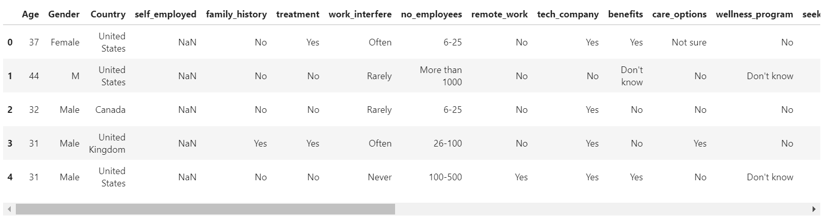
In this article, we are going to predict the mental health of Employees using various machine learning models. You can download the dataset from this link.
Library and Data Loading
import numpy as np
import pandas as pd
import matplotlib.pyplot as plt
import seaborn as sns
from scipy import stats
from scipy.stats import randint
# prep
from sklearn.model_selection import train_test_split
from sklearn import preprocessing
from sklearn.datasets import make_classification
from sklearn.preprocessing import binarize, LabelEncoder, MinMaxScaler
# models
from sklearn.linear_model import LogisticRegression
from sklearn.tree1 import DecisionTreeClassifier
from sklearn.ensemble import RandomForestClassifier, ExtraTreesClassifier
# Validation libraries
from sklearn import metrics
from sklearn.metrics import accuracy_score, mean_squared_error, precision_recall_curve
from sklearn.model_selection import cross_val_score1
#Neural Network
from sklearn.neural_network import MLPClassifier
from sklearn.model_selection import RandomizedSearchCV
#Bagging
from sklearn.ensemble import BaggingClassifier, AdaBoostClassifier
from sklearn.neighbors import KNeighborsClassifier
#Naive bayes
from sklearn.naive_bayes import GaussianNB
#Stacking
from mlxtend.classifier import StackingClassifier
#Get rid of bullshit
stk_list = ['A little about you', 'p']
train_df = train_df[~train_df['Gender'].isin(stk_list)]
print(train_df['Gender'].unique())
[‘female’ ‘male’ ‘trans’]
#complete missing age with mean
train_df['Age'].fillna(train_df['Age'].median(), inplace = True)
# Fill with media() values 120
s = pd.Series(train_df['Age'])
s[s<18] = train_df['Age'].median()
train_df['Age'] = s
s = pd.Series(train_df['Age'])
s[s>120] = train_df['Age'].median()
train_df['Age'] = s
#Ranges of Age
train_df['age_range'] = pd.cut(train_df['Age'], [0,20,30,65,100], labels=["0-20", "21-30", "31-65", "66-100"], include_lowest=True)
#There are only 0.014% of self employed so let's change NaN to NOT self_employed
#Replace "NaN" string from defaultString
train_df['self_employed'] = train_df['self_employed'].replace([defaultString], 'No')
print(train_df['self_employed'].unique())
[‘No’ ‘Yes’]
#There are only 0.20% of self work_interfere so let's change NaN to "Don't know
#Replace "NaN" string from defaultString
train_df['work_interfere'] = train_df['work_interfere'].replace([defaultString], 'Don't know' )
print(train_df['work_interfere'].unique())
#Encoding data
labelDict = {}
for feature in train_df:
le = preprocessing.LabelEncoder()
le.fit(train_df[feature])
le_name_mapping = dict(zip(le.classes_, le.transform(le.classes_)))
train_df[feature] = le.transform(train_df[feature])
# Get labels
labelKey = 'label_' + feature
labelValue = [*le_name_mapping]
labelDict[labelKey] =labelValue
for key, value in labelDict.items():
print(key, value)
#Get rid of 'Country'
train_df = train_df.drop(['Country'], axis= 1)
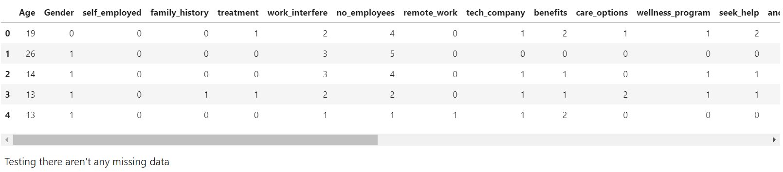
train_df.head()
#missing data
total = train_df.isnull().sum().sort_values(ascending=False)
percent = (train_df.isnull().sum()/train_df.isnull().count()).sort_values(ascending=False)
missing_data = pd.concat([total, percent], axis=1, keys=['Total', 'Percent'])
missing_data.head(20)
print(missing_data)
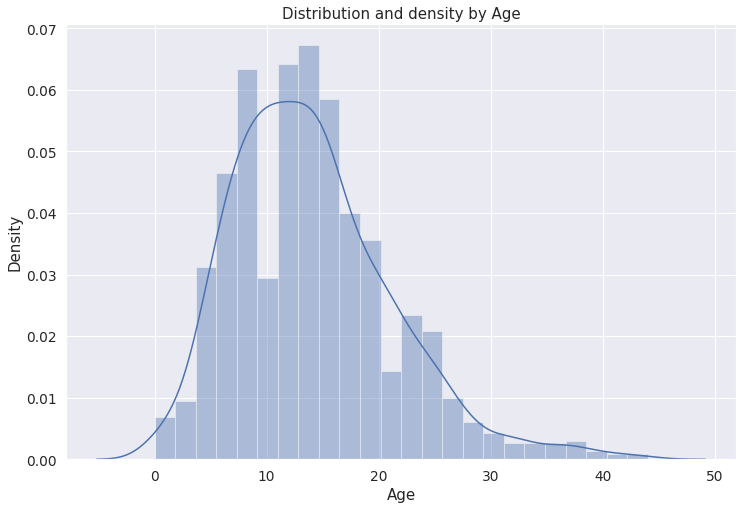
# Distribution and density by Age
plt.figure(figsize=(12,8))
sns.distplot(train_df["Age"], bins=24)
plt.title("Distribution and density by Age")
plt.xlabel("Age")
Text(0.5, 0, ‘Age’)
Inference: The above plot shows the Age column with respect to density. We can see that density is higher from Age 10 to 20 years in our dataset.
Inference: Treatment 0 means treatment is not necessary 1 means it is. First Barplot shows that from age 0 to 10-year treatment is not necessary and is needed after 15 years.
plt.figure(figsize=(12,8))
labels = labelDict['label_Gender']
j = sns.countplot(x="treatment", data=train_df)
j.set_xticklabels(labels)
plt.title('Total Distribution by treated or not')
Text(0.5, 1.0, ‘Total Distribution by treated or not’)
Inference: Here we can see that more males are treated as compared to females in the dataset.
o = labelDict['label_age_range']
j = sns.factorplot(x="age_range", y="treatment", hue="Gender", data=train_df, kind="bar",  ci=None, size=5, aspect=2, legend_out = True)
j.set_xticklabels(o)
plt.title('Probability of mental health condition')
plt.ylabel('Probability x 100')
plt.xlabel('Age')
new_labels = labelDict['label_Gender']
for t, l in zip(j._legend.texts, new_labels): t.set_text(l)
j.fig.subplots_adjust(top=0.9,right=0.8)
plt.show()
Inference: This barplot shows the mental health of females, males, and transgender according to different age groups. we can analyze that from the age group of 66 to 100, mental health is very high in females as compared to another gender. And from age 21 to 64, mental health is very high in transgender as compared to males.
o = labelDict['label_family_history']
j = sns.factorplot(x="family_history", y="treatment", hue="Gender", data=train_df, kind="bar", ci=None, size=5, aspect=2, legend_out = True)
j.set_xticklabels(o)
plt.title('Probability of mental health condition')
plt.ylabel('Probability x 100')
plt.xlabel('Family History')
new_labels = labelDict['label_Gender']
for t, l in zip(g._legend.texts, new_labels): t.set_text(l)
j.fig.subplots_adjust(top=0.9,right=0.8)
plt.show()
o = labelDict['label_care_options']
j = sns.factorplot(x="care_options", y="treatment", hue="Gender", data=train_df, kind="bar", ci=None, size=5, aspect=2, legend_out = True)
j.set_xticklabels(o)
plt.title('Probability of mental health condition')
plt.ylabel('Probability x 100')
plt.xlabel('Care options')
new_labels = labelDict['label_Gender']
for t, l in zip(g._legend.texts, new_labels): t.set_text(l)
j.fig.subplots_adjust(top=0.9,right=0.8)
plt.show()
Inference: In the dataset, for those who are having a family history of mental health problems, the Probability of mental health will be high. So here we can see that probability of mental health conditions for transgender is almost 90% as they have a family history of medical health conditions.
Inference: This barplot shows health status with respect to care options. In the dataset, for Those who are not having care options, the Probability of mental health situation will be high. So here we can see that the mental health of transgender is very high who have not care options and low for those who are having care options.
o = labelDict['label_benefits']
j = sns.factorplot(x="care_options", y="treatment", hue="Gender", data=train_df, kind="bar", ci=None, size=5, aspect=2, legend_out = True)
j.set_xticklabels(o)
plt.title('Probability of mental health condition')
plt.ylabel('Probability x 100')
plt.xlabel('Benefits')
new_labels = labelDict['label_Gender']
for t, l in zip(j._legend.texts, new_labels): t.set_text(l)
j.fig.subplots_adjust(top=0.9,right=0.8)
plt.show()
Inference: This barplot shows the probability of health conditions with respect to Benefits. In the dataset, for those who are not having any benefits, the Probability of mental health conditions will be high. So here we can see that probability of mental health conditions for transgender is very high who have not getting any benefits. and probability is low for those who are having benefits options.
o = labelDict['label_work_interfere']
j = sns.factorplot(x="work_interfere", y="treatment", hue="Gender", data=train_df, kind="bar", ci=None, size=5, aspect=2, legend_out = True)
j.set_xticklabels(o)
plt.title('Probability of mental health condition')
plt.ylabel('Probability x 100')
plt.xlabel('Work interfere')
new_labels = labelDict['label_Gender']
for t, l in zip(g._legend.texts, new_labels): t.set_text(l)
j.fig.subplots_adjust(top=0.9,right=0.8)
plt.show()
Inference: This barplot shows the probability of health conditions with respect to work interference. For those who are not having any work interference, the Probability of mental health conditions will be very less. and probability is high for those who are having work interference rarely.
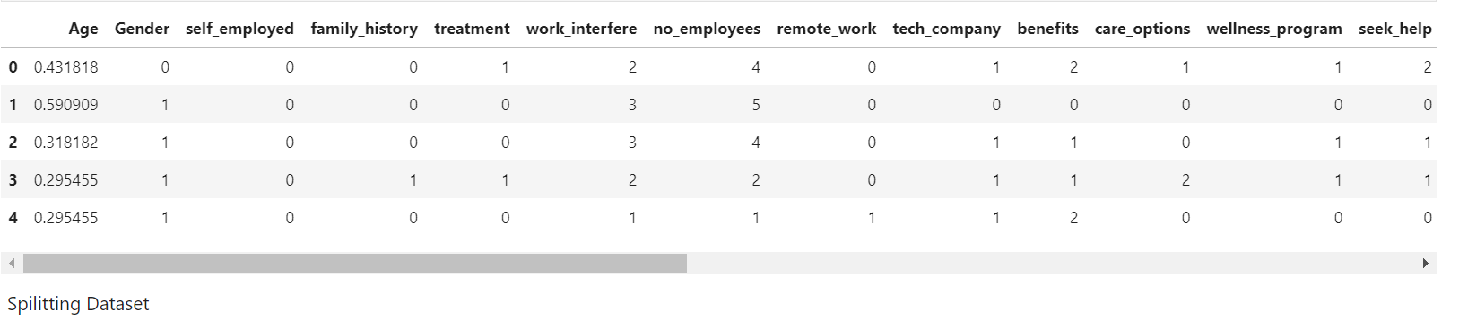
Scaling and Fitting
# Scaling Age
scaler = MinMaxScaler()
train_df['Age'] = scaler.fit_transform(train_df[['Age']])
train_df.head()
# define X and y
feature_cols1 = ['Age', 'Gender', 'family_history', 'benefits', 'care_options', 'anonymity', 'leave', 'work_interfere']
X = train_df[feature_cols1]
y = train_df.treatment
X_train1, X_test1, y_train1, y_test1 = train_test_split(X, y, test_size=0.30, Random_state1=0)
# Create dictionaries for final graph
# Use: methodDict['Stacking'] = accuracy_score
methodDict = {}
rmseDict = ()
forest = ExtraTreesClassifier(n_estimators=250,
                              Random_state1=0)
forest.fit(X, y)
importances = forest.feature_importances_
std = np.std([tree1.feature_importances_ for tree in forest.estimators_],
             axis=0)
indices = np.argsort(importances)[::-1]
labels = []
for f in Range(x.shape[1]):
    labels.append(feature_cols1[f])
plt.figure(figsize=(12,8))
plt.title("Feature importances")
plt.bar(range(X.shape[1]), importances[indices],
       color="r", yerr=std[indices], align="center")
plt.Xticks(range(X.shape[1]), labels, rotation='vertical')
def tuningCV(knn):
    k_Range = list(Range(1, 31))
    k_scores = []
    for k in k_range:
        knn = KNeighborsClassifier(n_neighbors=k)
        scores = cross_val_score1(knn, X, y, cv=10, scoring='accuracy')
        k_scores.append(scores.mean())
    print(k_scores)
    plt.plot(k_Range, k_scores)
    plt.xlabel('Value of K for KNN')
    plt.ylabel('Cross-Validated Accuracy')
    plt.show()
Tuning with GridSearchCV
def tuningGridSerach(knn):

    k_Range = list(range(1, 31))
    print(k_Range)

    param_grid = dict(n_neighbors=k_range)
    print(param_grid)

    grid = GridSearchCV(knn, param_grid, cv=10, scoring='accuracy')

    grid.fit(X, y)
    grid.grid_scores1_

    print(grid.grid_scores_[0].parameters)
    print(grid.grid_scores_[0].cv_validation_scores)
    print(grid.grid_scores_[0].mean_validation_score)
    grid_mean_scores1 = [result.mean_validation_score for result in grid.grid_scores_]
    print(grid_mean_scores1)
    # plot the results
    plt.plot(k_Range, grid_mean_scores1)
    plt.xlabel('Value of K for KNN')
    plt.ylabel('Cross-Validated Accuracy')
    plt.show()
    # examine the best model
    print('GridSearch best score', grid.best_score_)
    print('GridSearch best params', grid.best_params_)
    print('GridSearch best estimator', grid.best_estimator_)
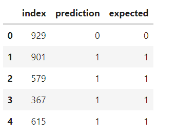
The final prediction consists of 0 and 1. 0 means the person is not needed any mental health treatment and 1 means the person is needed mental health treatment.
Conclusion
After using all these Employee records, we are able to build various machine learning models. From all the models, ADA–Boost achieved 81.75% accuracy with an AUC of 0.8185 along with that we were able to draw some insights from the data via data analysis and visualization.
The media shown in this article is not owned by Analytics Vidhya and is used at the Author’s discretion.
I currently working as an Assistant professor in the Information technology department at SAL COLLEGE OF ENGINEERING, AHMEDABAD .I am currently doing Ph.D. in Medical Image processing. My research interest are computer vision, deep learning, machine learning, database etc.

.png)
.png)
.png)
.png)
.png)
.png)
.png)
.png)
.png)
.png)
.png)
.png)
.png)
.png)
.png)
.png)
.png)
.png)
.png)
.png)
.png)
.png)
.png)
.png)