If you have just started to learn machine learning, chances are you have already heard about a Decision Tree. While you may not presently be aware of its working, know that you have definitely used it in some form or the other. Decision Trees have long powered the backend of some of the most popular services available globally. While there are better alternatives available now, decision trees still hold their importance in the world of machine learning.
To give you a context, a decision tree is a supervised machine learning algorithm used for both classification and regression tasks. Decision tree analysis involves different choices and their possible outcomes, which help make decisions easily based on certain criteria, as we’ll discuss later in this blog.
In this article, we’ll go through what decision trees are in machine learning, how the decision tree algorithm works, their advantages and disadvantages, and their applications.
Table of contents
What is Decision Tree?
A decision tree is a non-parametric machine learning algorithm, which means that it makes no assumptions about the relationship between input features and the target variable. Decision trees can be used for classification and regression problems. A decision tree resembles a flow chart with a hierarchical tree structure consisting of:
- Root node
- Branches
- Internal nodes
- Leaf nodes

Types of Decision Trees
There are two different kinds of decision trees: classification and regression trees. These are sometimes both called CART (Classification and Regression Trees). We will talk about both briefly in this section.
- Classification Trees: A classification tree predicts categorical outcomes. This means that it classifies the data into categories. The tree will then guess which category the new sample belongs in. For example, a classification tree may output whether an email is “Spam” or “Not Spam” based on the features of the sender, subject and content.
- Regression Trees: A regression tree is used when the target variable is continuous. This means predicting a numerical value as opposed to a categorical value. This is done by averaging the values of that leaf. For example, a regression tree could predict the highest price of a house; the features could be size, area, number of bedrooms, and location.
This algorithm typically utilizes ‘Gini impurity’ or ‘Entropy’ to identify the ideal attribute for a node split. Gini impurity measures how often a randomly chosen attribute is misclassified. The lower the value, the better the split will be for that attribute. Entropy is a measure of disorder or randomness in the dataset, so the lower the value of entropy for an attribute, the more desirable it is for tree split, and will lead to more predictable splits.
Similarly, in practice, we’ll choose the type by using either DecisionTreeClassifier or DecisionTreeRegressor for classification and regression:
from sklearn.tree import DecisionTreeClassifier, DecisionTreeRegressor
# Example classifier (e.g., predict emails are spam or not)
clf = DecisionTreeClassifier(max_depth=3, random_state=42)
# Example regressor (e.g., predict house prices)
reg = DecisionTreeRegressor(max_depth=3)
Information Gain and Gini Index in Decision Tree
Up to now, we have discussed the basic intuition and approach of how a decision tree works. So, now let’s discuss the selection measures of the decision tree, which ultimately help in selecting the ideal node for the splitting process. For that, we have two popular approaches we’ll discuss below:
1. Information Gain
Information Gain is the measure of effectiveness of a particular attribute in reducing the entropy in the dataset. This helps in selecting the most informative features for splitting the data, leading to a more accurate & efficient model.
So, suppose S is a set of instances and A is an attribute. Sv is the subset of S, and V represents an individual value of that attribute. A can take one value from the set of (A), which is the set of all possible values for that attribute.

Entropy: In the context of decision trees, entropy is the measure of disorder or randomness in the dataset. It is maximum when the classes are evenly distributed and decreases when the distribution becomes more homogeneous. So, a node with low entropy means classes are mostly similar or pure within that node.
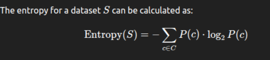
Where P(c) is the probability of classes in the set S and C is the set of all classes.
Example: If we want to decide whether to play tennis or not based on the weather conditions: Outlook and Temperature.
Outlook has 3 values: Sunny, Overcast, Rain
Temperature has 3 values: Hot, Mild, Cold, and
Play Tennis outcome has 2 values: Yes or No.
| Outlook | Play Tennis | Count |
|---|---|---|
| Sunny | No | 3 |
| Sunny | Yes | 2 |
| Overcast | Yes | 4 |
| Rain | No | 1 |
| Rain | Yes | 4 |
Calculating Information Gain
Now we’ll calculate the Information when the split is based on Outlook.
Step 1: Entropy of Entire Dataset S
So, the total number of instances in S is 14, and their distribution is:
- Yes: 9
- No: 5
The entropy of S will be:
Entropy(S) = -(9/14 log2(9/14) + 5/14 log2(5/14) = 0.94
Step 2: Entropy for the subset based on outlook
Now, let’s break the data points into subsets based on the Outlook distribution, so:
Sunny (5 records: 2 Yes and 3 No):
Entropy(Sunny)= -(⅖ log2(⅖)+ ⅗ log2(⅗)) =0.97
Overcast (4 records: 4 Yes, 0 No):
Entropy(Overcast) = 0 (as it’s a pure attribute, as all values are the same)
Rain (5 records: 4 Yes, 1 No):
Entropy(Rain) = -(⅘ log2(⅘)+ ⅕ log2(⅕)) = 0.72
Step 3: Calculate Information Gain
Now we’ll calculate information gain based on outlook:
Gain(S,Outlook) = Entropy(S) – (5/14 * Entropy(Sunny) + 4/14 * Entropy(Overcast) + 5/14 * Entropy(Rain))
Gain(S,Outlook) = 0.94-(5/14 * 0.97+ 4/14 * 0+ 5/14 * 0.72) = 0.94-0.603=0.337
So the Information Gain for the Outlook attribute is 0.337
The Outlook attribute here indicates it’s somewhat effective in deriving the solution. However, it still leaves some uncertainty about the right outcome.
2. Gini Index
Just like Information Gain, the Gini Index is used to decide the best feature for splitting the data, but it operates differently. Gini Index is a metric to measure how often a randomly chosen element would be incorrectly identified or impure (how mixed the classes are in a subset of data). So, the higher the value of the Gini Index for an attribute, the less likely it is to be chosen for the data split. Therefore, an attribute with a higher Gini index value is preferred in such decision trees.

Where:
m is the number of classes in the dataset and
P(i) is the probability of class i in the dataset S.
For example, if we have a binary classification problem with classes “Yes” and “No”, then the probability of each class is the fraction of instances in each class. The Gini Index ranges from 0, as perfectly pure, and 0.5, as maximum impurity for binary classification.
Therefore, Gini=0 means that all instances in the subset belong to the same class, and Gini=0.5 means; the instances are equal proportions of all classes.
Example: If we want to decide whether to play tennis or not based on the weather conditions: Outlook, and Temperature.
Outlook has 3 values: Sunny, Overcast, Rain
Temperature has 3 values: Hot, Mild, Cold, and
Play Tennis outcome has 2 values: Yes or No.
|
Outlook |
Play Tennis |
Count |
|
Sunny |
No |
3 |
|
Sunny |
Yes |
2 |
|
Overcast |
Yes |
4 |
|
Rain |
No |
1 |
|
Rain |
Yes |
4 |
Calculating Gini Index
Now we’ll calculate the Gini Index when the split is based on Outlook.
Step 1: Gini Index of Entire Dataset S
So, the total number of instances in S is 14, and their distribution is:
- Yes: 9
- No: 5
The Gini Index of S will be:
P(Yes) = 9/14, P(No) = 5.14
Gain(S)= 1-((9/14)^2 + (5/14)^2)
Gain(S) = 1-(0.404_0.183) = 1- 0.587 = 0.413
Step 2: Gini Index for each subset based on Outlook
Now, let’s break the data points into subsets based on the Outlook distribution, so:
Sunny(5 records: 2 Yes and 3 No):
P(Yes)=⅖, P(No) = ⅗
Gini(Sunny) = 1-((⅖)^2 +(⅗)^2) = 0.48
Overcast (4 records: 4 Yes, 0 No):
Since all instances in this subset are “Yes”, the Gini Index is:
Gini(Overcast) = 1-(4/4)^2 +(0/4)^2)= 1-1= 0
Rain (5 records: 4 Yes, 1 No):
P(Yes)=⅘, P(No)=⅕
Gini(Rain) = 1-((⅘ )^2 +⅕ )^2) = 0.32
Overcast (4 records: 4 Yes, 0 No):
Since all instances in this subset are “Yes”, the Gini Index is:
Gini(Overcast) = 1-(4/4)^2 +(0/4)^2)= 1-1= 0
Rain (5 records: 4 Yes, 1 No):
P(Yes)=⅘, P(No)=⅕
Gini(Rain) = 1-((⅘ )^2 +⅕ )^2) = 0.32
Step 3: Weighted Gini Index for Split
Now, we calculate the Weighted Gini Index for the split based on Outlook. This will be the Gini Index for the entire dataset after the split.
Weighted Gini(S,Outlook)= 5/14 * Gini(Sunny) + 4/14 * Gini(Overcast) + 5/14 * (Gini(Rain)
Weighted Gini(S,Outlook)= 5/14 * 0.48+ 4/14 *0 + 5/14 * 0.32 = 0.286
Step 4: Gini Gain
Gini Gain will be calculated as the reduction in the Gini Index after the split. So,
Gini Gain(S,Outlook)=Gini(S)−Weighted Gini(S,Outlook)
Gini Gain(S,Outlook) = 0.413 – 0.286 = 0.127
So, the Gini Gain for the Outlook attribute is 0.127. This means that by using Outlook as a splitting node, the impurity of the dataset can be reduced by 0.127. This indicates the effectiveness of this feature in classifying the data.
How Does a Decision Tree Work?
As discussed, a decision tree is a supervised machine learning algorithm that can be used for both regression and classification tasks. A decision tree starts with the selection of a root node using one of the splitting criteria – information gain or gini index. So, building a decision tree involves recursive splitting the training data until the probability of distinction of outcomes in each branch becomes maximum. The decision tree algorithm proceeds top-down from the root. Here is how it works:
- Start with the Root Node with all training samples.
- Choose the best attribute to split the data. The best feature for the split will be the one that gives the most number of pure child nodes(meaning where the data points belong to the same class). This can be measured either by information gain or the Gini index.
- Splitting the data into small subsets according to the chosen feature with max information gain or minimum Gini index, creating further pure child nodes until the final results are homogenous or from the same class.
- The final step stops the tree from further growing when the condition is met, known as the storing criteria. It occurs if or when:
- All the data in the node belongs to the same class or is a pure node.
- No further split remains.
- A maximum depth of the tree is reached.
- The minimum number of nodes becomes the leaf and is labelled as the predicted class/value for a particular region or attribute.
Recursive Partitioning
This top-down process is called recursive partitioning. It is also known as greedy algorithm, as at each step, the algorithm picks the best split based on the current data. This approach is efficient but does not ensure a generalized optimal tree.
For example, think of a decision tree for a coffee decision. The root node asks, “Time of Day?”; if it’s morning, it asks “Tired?”; if yes, it leads to “Drink Coffee,” else to “No Coffee.” A similar branch exists for the afternoon. This illustrates how a tree makes sequential decisions until reaching a final answer.
For this example, the tree starts with “Time of day?” at the root. Depending on the answer to this, the next node will be “Are you tired?”. Finally, the leaf gives the final class or decision “Drink Coffee” or “No Coffee”.
Now, as the tree grows, each split aims to create a pure child node. If splits stop early (due to depth limit or small sample size), the leaf may be impure, containing a mix of classes; then its prediction may be the majority class in that leaf.
And if the tree grows very large, we have to add a depth limit or pruning (meaning removing the branches that are not important) to prevent overfitting and to control tree size.
Advantages and disadvantages of decision trees
Decision trees have many strengths that make them a popular choice in machine learning, although they have pitfalls. In this section, we will talk about some of the greatest advantages and disadvantages of decision trees:
Advantages
- Easy to understand and interpret: Decision trees are very intuitive and can be visualized as flow charts. Once a tree is built or completed, one can easily see which feature leads to which prediction. This makes a model more transparent.
- Handle both numerical and categorical data: Decision trees handle both categorical and numerical data by default. They don’t require any encoding techniques, which makes them even more flexible, meaning we can feed mixed data types without extensive data preprocessing.
- Captures non-linear relations in the data: Decision trees are also known as they are able to analyze and understand the complex hidden patterns from data, so they can capture the non-linear relationships between input features and target variables.
- Fast and Scalable: Decision trees take very little time while training and can handle datasets with reasonable efficiency as they are non-parametric.
- Minimal data preparation: Decision trees don’t require feature scaling because they split on actual categories means there is less need to do that externally; most of the scaling is handled internally.
Disadvantages
- Overfitting: As the tree grows deeper, a decision tree easily overfits on the training data. This means the final model will not be able to perform well due to the lack of generalization on test or unseen real-world data
- Instability: The efficiency of the decision tree depends on the node it chooses to split the data to find a pure node. But small changes in the training set or a wrong decision while choosing the node can lead to a very different tree. As a result, the outcome of the tree is unstable.
- Complexity increases as the depth of the tree increases: Deep trees with many levels also require more memory and time to evaluate, along with the issue of overfitting, as discussed.
Applications of Decision Trees
Decision Trees are popular in practice across the machine learning and data science fields due to their interpretability and flexibility. Here are some real-world examples:
- Recommendation Systems: A decision tree can provide recommendations to a user on an e-commerce or media site by analyzing that user’s activity and content preferences based on their behavior. Based on all the patterns and splits in a tree, it will suggest particular products or content that the user is likely interested in. For example, for an online retailer, a decision tree can be used to classify the product category of a user based on their activity online.
- Fraud Detection: Decision trees are often used in financial fraud detection to sort suspicious transactions. In this case, the tree can split on things like transaction amount, transaction location, frequency of transactions, character traits and a lot more to classify if the activity is fraudulent.
- Marketing and Customer Segmentation: The marketing teams of firms can use decision trees to segment or organize customers. In this case, a decision tree could be used to categorize if the customer would be likely to respond to a campaign or if they were more likely to churn based on historical patterns in the data.
These examples demonstrate the broad use case for decision trees, they can be used in both classification and regression tasks in fields varying from recommendation algorithms to marketing to engineering.
Hello! I'm Vipin, a passionate data science and machine learning enthusiast with a strong foundation in data analysis, machine learning algorithms, and programming. I have hands-on experience in building models, managing messy data, and solving real-world problems. My goal is to apply data-driven insights to create practical solutions that drive results. I'm eager to contribute my skills in a collaborative environment while continuing to learn and grow in the fields of Data Science, Machine Learning, and NLP.


