How to Improve Class Imbalance using Class Weights in Machine Learning?

Class imbalance often hinders accurate predictions in machine learning models, a common challenge in binary classification tasks. Class imbalance occurs when one class significantly outweighs the other regarding data samples, leading to biased predictions. One effective technique for addressing class imbalance is the strategic use of class weights. Class weights assign higher weights to the minority class, allowing the model to pay more attention to its patterns and reducing bias towards the majority class. This article explores the concept of class weights in machine learning, their significance in handling class imbalances, and practical implementation strategies to improve model performance in imbalanced datasets.

Learning Objective

• Understand how class weight for imbalanced data optimization works.
• Discover how to implement the same in logistic regression or any other algorithm using sklearn.
• Learn how class weights can help overcome class imbalance data problems without using any sampling method.

This article was published as a part of the Data Science Blogathon.

What is Class Imbalance?

Class imbalance is a problem that occurs in machine learning classification problems. It merely tells that the target class’s frequency is highly imbalanced, i.e., the occurrence of one of the classes is very high compared to the other classes present. In other words, there is a bias or skewness towards the majority class present in the target. Suppose we consider a binary classification where the majority target class has 10000 rows, and the minority target class has only 100 rows. In that case, the ratio is 100:1, i.e., for every 100 majority class, there is only one minority class present. This problem is what we refer to as class imbalance. Some general areas where we can find such data are fraud detection, churn prediction, medical diagnosis, e-mail classification, etc.

To understand class imbalance properly, we will be working on a dataset from the medical domain. Here, we have to predict whether a person will have a heart stroke based on the given attributes (independent variables). We are using the cleaned version of the data to skip the cleaning and preprocessing of the data.

In the image below, you can see the distribution of our target variable. (The distribution may differ on the repl as the dataset may be updated over time.)

Python Code

import pandas as pd
import seaborn as sns
import matplotlib.pyplot as plt
data = pd.read_csv('healthcare-dataset-stroke-data.csv')
#Ploting barplot for target 
plt.figure(figsize=(10,6))
g = sns.barplot(data['stroke'], data['stroke'], palette='Set1', estimator=lambda x: len(x) / len(data) )

#Anotating the graph
for p in g.patches:
        width, height = p.get_width(), p.get_height()
        x, y = p.get_xy() 
        g.text(x+width/2, 
               y+height, 
               '{:.0%}'.format(height), 
               horizontalalignment='center',fontsize=15)

#Setting the labels
plt.xlabel('Heart Stroke', fontsize=14)
plt.ylabel('Precentage', fontsize=14)
plt.title('Percentage of patients will/will not have heart stroke', fontsize=16)
plt.show()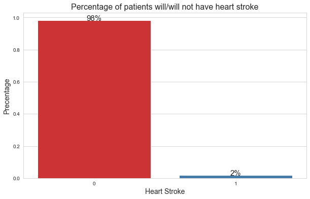

Here,

• 0: signifies that the patient didn’t have a heart stroke.
• 1: signifies that the patient had a heart stroke.

From the distribution, we can see that only 2% of patients had a heart stroke. So, this is a classic class imbalance problem.

Why is it Essential to Deal with Class Imbalance?

So far, we have the intuition about class imbalance. But why is it necessary to overcome this, and what problems does it create while modelling with such data?

Most machine learning algorithms assume that the data is evenly distributed within classes. In the case of class imbalance problems, the extensive issue is that the algorithm will be more biased towards predicting the majority class (no heart stroke in our case). The algorithm will not have enough data to learn the patterns in the minority class (heart stroke).

Example

You have shifted from your hometown to a new city and have been living here for the past month. When it comes to your hometown, you will be very familiar with all the locations like your home, routes, essential shops, tourist spots, etc., because you spent your whole childhood there. But when it comes to the new city, you would not have many ideas about where each location exactly is, and the chances of taking the wrong routes and getting lost will be very high. Here, your hometown is your majority class, and the new city is the minority class.

Similarly, this happens in class imbalance. The model has adequate information about the majority class but insufficient information about the minority class. That is why there will be high misclassification errors for the minority class.

Note: We will use the F1 score as the metric to check the model’s performance, not accuracy.

The reason is if we create a dumb model that predicts every new training data as 0 (no heart stroke) even then we will get very high accuracy because the model is biased towards the majority class. Here, the model is heavily accurate but does not serve any value to our problem statement. That is why we will use the f1 score as the evaluation metric. The F1 score is nothing but the harmonic mean of precision and recall. However, the evaluation metric is chosen based on the business problem and the type of error we want to reduce. But, the f1 score is the go-to metric for class imbalance problems.

Formula for f1-score

f1 score = 2*(precision*recall)/(precision+recall)

Let’s confirm this by training a model based on the model of the target variable on our heart stroke data and check what scores we get:

#Training the model using mode of target
from sklearn.metrics import f1_score, accuracy_score, confusion_matrix
pred_test = []
for i in range (0, 13020):
    pred_test.append(y_train.mode()[0])

#Printing f1 and accuracy scores    
print('The accuracy for mode model is:', accuracy_score(y_test, pred_test))
print('The f1 score for the model model is:',f1_score(y_test, pred_test))

#Ploting the cunfusion matrix
conf_matrix(y_test, pred_test)

The accuracy for the mode model is: 0.9819508448540707

The f1 score for the mode model is: 0.0

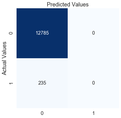
Here, the mode model’s accuracy on the testing data is 0.98, an excellent score. However, the f1 score is zero, indicating that the model performs poorly in the minority class. We can confirm this by looking at the confusion matrix.

The mode model predicts every patient as 0 (no heart stroke). According to this model, no matter what symptoms a patient has, he/she will never have a heart stroke. Does using this model make any sense?

Now that we understand class imbalance and how it plagues our model performance, we will shift our focus to class weights and how class weights can help improve the model’s performance.

Also Read: 10 Techniques to Solve Imbalanced Classes in Machine Learning

What are Class Weights?

Most machine learning algorithms are not very useful with biased class data. But, we can modify the current training algorithm to consider the skewed distribution of the classes. This can be achieved by giving weight to the majority and minority classes. The difference in weights will influence the classification of the classes during the training phase. The whole purpose is to penalize the misclassification made by the minority class by setting a higher class weight and simultaneously reducing the weight for the majority class.

Example of Class Weights

Please think of it this way: the last month you spent in the new city, instead of going out when needed, you spent the whole month exploring the city. You spent more time understanding the city routes and places the entire month. Giving more research time will help you know the new city better, and the chances of getting lost will be reduced. And this is precisely how class weights work. During the training, we gave more weightage to the minority class in the cost function of the algorithm so that it could provide a higher penalty to the minority class, and the algorithm could focus on reducing the errors for the minority class.

Note: There is a threshold at which you should increase and decrease the class weights for the minority and majority classes, respectively. If you give very high-class weights to the minority class, the algorithm will likely become biased towards the minority class, increasing the errors in the majority class.

Most sklearn classifier modelling libraries and boosting-based libraries like LightGBM and catboost have an in-built parameter “class_weight”, which helps us optimize the scoring for the minority class, just as we have learned so far.

By default, the value of class_weight=None, i.e. both the classes have been given equal weights. Other than that, we can either give it a ‘balanced’ rating or pass a dictionary that contains manual weights for both classes.

When the class_weights = ‘balanced’, the model automatically assigns the class weights inversely proportional to their respective frequencies.

Formula of Class Weights

wj=n_samples / (n_classes * n_samplesj)

Here,

• wj is the weight for each class(j signifies the class)
• n_samplesis the total number of samples or rows in the dataset
• n_classesis the total number of unique classes in the target
• n_samplesjis the total number of rows of the respective class

For our heart stroke example:

• n_samples=  43400,  n_classes= 2(0&1), n_sample0= 42617, n_samples1= 783
• Weights for class 0:
• w0=  43400/(2*42617) = 0.509
• Weights for class 1:
• w1= 43400/(2*783) = 27.713

I hope this makes it clearer that class_weight = ‘balanced’ helps us give higher weights to the minority class and lower weights to the majority class.

Although passing value as ‘balanced’ gives good results in most cases, sometimes, for extreme class imbalance, we can try giving weights manually. Later, we will see how we can find the optimal value for the class weights in Python.

Class Weights in Logistic Regression

We can modify every machine learning algorithm by adding different class weights to its cost function, but here, we will focus on logistic regression.

For the logistic regression, we use log loss as the cost function. We don’t use the mean squared error as the cost function for the logistic regression because instead of fitting a straight line, we use the sigmoid curve as the prediction function. Squaring the sigmoid function will result in a non-convex curve, which will cause the cost function to have a lot of local minima, and converging to the global minima using gradient descent is extremely difficult. But log loss forms a convex function, and we only have one minimum to converge.

Formula for Log Loss

Here,

• N is the number of values
• yi is the actual value of the target class
• yi is the predicted probability of the target class

Let’s form a pseudo table that has actual predictions, predicted probabilities, and calculated cost using the log loss formula:

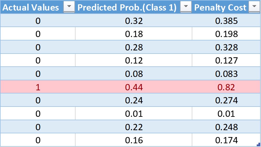
This table has ten observations, nine from class 0 and 1 from class 1. In the next column, we have the predicted probabilities for each observation. And finally, using the log loss formula, we have the cost penalty.

After adding the weights to the cost function, the modified log loss function is:

Here,

• w0 is the class weight for class 0
• w1 is the class weight for class 1

Now, we will add the weights and see what difference it will make to the cost penalty.

For the values of the weights, we will be using the class_weights=’balanced’ formula.

• w0= 10/(2*1) = 5
• w1= 10/(2*9) = 0.55

Calculating the cost for the first value in the table:

• Cost = -(5(0*log(0.32) + 0.55(1-0)*log(1-0.32))
• = -(0 + 0.55*log(.68))
• = -(0.55*(-0.385))
• = 0.211

Similarly, we can calculate the weighted cost for each observation, and the updated table is:

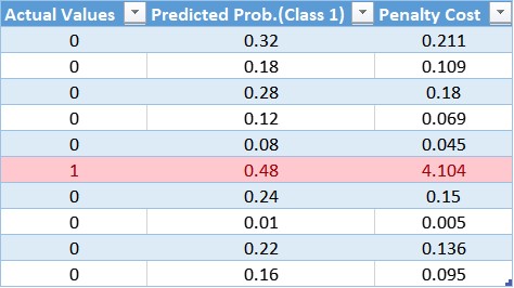
Through the table, we can confirm the small weight applied to the cost function for the majority class, which results in a smaller error value and, in turn, less update to the model coefficients. A more considerable weight value is applied to the cost function for the minority class, resulting in a larger error calculation and, in turn, more updates to the model coefficients. This way, we can shift the bias of the model so that it could also reduce the errors of the minority class.

Conclusion

• Small weights result in a small penalty and a small update to the model coefficients.
• Large weights result in a large penalty and a large update to the model coefficients.
  

Implementation in Python

Here, we will use the same heart-stroke data for our predictions. First, we will train a simple logistic regression, then implement the weighted logistic regression with class_weights as ‘balanced’. Finally, we will try to find the optimal value of class weights using a grid search. The metric we try to optimize will be the F1 score.

1. Simple Logistic Regression

Here, we are using the sklearn library to train our model, and we are using the default logistic regression. By default, the algorithm will give equal weights to both the classes.

#importing and training the model
from sklearn.linear_model import LogisticRegression
lr = LogisticRegression(solver='newton-cg')
lr.fit(x_train, y_train)

# Predicting on the test data
pred_test = lr.predict(x_test)

#Calculating and printing the f1 score 
f1_test = f1_score(y_test, pred_test)
print('The f1 score for the testing data:', f1_test)

# Function to create a confusion matrix 
def conf_matrix(y_test, pred_test):    
    
    # Creating a confusion matrix
    con_mat = confusion_matrix(y_test, pred_test)
    con_mat = pd.DataFrame(con_mat, range(2), range(2))
   
    #Ploting the confusion matrix
    plt.figure(figsize=(6,6))
    sns.set(font_scale=1.5) 
    sns.heatmap(con_mat, annot=True, annot_kws={"size": 16}, fmt='g', cmap='Blues', cbar=False)
    
#Calling function 
conf_matrix(y_test, pred_test)

The f1-score for the testing data: 0.0

We got the F1 score as 0 for a simple logistic regression model. Looking at the confusion matrix, we can confirm that our model predicts that every observation will not result in a heart stroke. This model is not any better than the mode model we created earlier. Let’s try adding some weight to the minority class and see if that helps.

2. Logistic Regression (class_weight=’balanced’)

We have added the class_weight parameter to our logistic regression algorithm, and the value we passed is ‘balanced’.

#importing and training the model
from sklearn.linear_model import LogisticRegression
lr = LogisticRegression(solver='newton-cg', class_weight='balanced')
lr.fit(x_train, y_train)

# Predicting on the test data
pred_test = lr.predict(x_test)

#Calculating and printing the f1 score 
f1_test = f1_score(y_test, pred_test)
print('The f1 score for the testing data:', f1_test)

#Ploting the confusion matrix
conf_matrix(y_test, pred_test)

The f1-score for the testing data: 0.10098851188885921

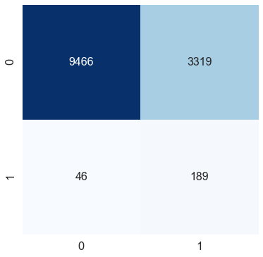
Adding a single class weight parameter to the logistic regression function improved the f1 score by 10 per cent. We can see in the confusion matrix that even though the misclassification for class 0 (no heart stroke) has increased, the model can capture class 1 (heart stroke) pretty well.

Can we improve the metric any further just by changing class weights?

3. Logistic Regression (manual class weights)

Finally, we are using grid search to find optimal weights with the highest score. We will search for weights between 0 and 1. If we give n as the weight for the minority class, the majority class will get 1-n as the weight.

The magnitude of the weights is not very large here, but the ratio of weights between the majority and minority classes will be very high.

Example:

• w1 = 0.95
• w0 = 1 – 0.95 = 0.05
• w1:w0 = 19:1

So, the weights for the minority class will be 19 times higher than the majority class.

from sklearn.model_selection import GridSearchCV, StratifiedKFold
lr = LogisticRegression(solver='newton-cg')

#Setting the range for class weights
weights = np.linspace(0.0,0.99,200)

#Creating a dictionary grid for grid search
param_grid = {'class_weight': [{0:x, 1:1.0-x} for x in weights]}

#Fitting grid search to the train data with 5 folds
gridsearch = GridSearchCV(estimator= lr, 
                          param_grid= param_grid,
                          cv=StratifiedKFold(), 
                          n_jobs=-1, 
                          scoring='f1', 
                          verbose=2).fit(x_train, y_train)

#Ploting the score for different values of weight
sns.set_style('whitegrid')
plt.figure(figsize=(12,8))
weigh_data = pd.DataFrame({ 'score': gridsearch.cv_results_['mean_test_score'], 'weight': (1- weights)})
sns.lineplot(weigh_data['weight'], weigh_data['score'])
plt.xlabel('Weight for class 1')
plt.ylabel('F1 score')
plt.xticks([round(i/10,1) for i in range(0,11,1)])
plt.title('Scoring for different class weights', fontsize=24)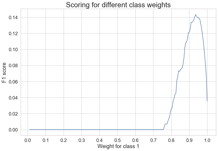

The graph shows that the highest value for the minority class is peaking at about 0.93 class weight.

Using grid search, we got the best class weight: 0.06467 for class 0 (majority class) and 1: 0.93532 for class 1 (minority class).

Now that we have our best class weights using stratified cross-validation and grid search, we will see the performance on the test data.

#importing and training the model
from sklearn.linear_model import LogisticRegression
lr = LogisticRegression(solver='newton-cg', class_weight={0: 0.06467336683417085, 1: 0.9353266331658292})
lr.fit(x_train, y_train)

# Predicting on the test data
pred_test = lr.predict(x_test)

#Calculating and printing the f1 score 
f1_test = f1_score(y_test, pred_test)
print('The f1 score for the testing data:', f1_test)

#Ploting the confusion matrix
conf_matrix(y_test, pred_test)

The f1-score for the testing data: 0.1579371474617244

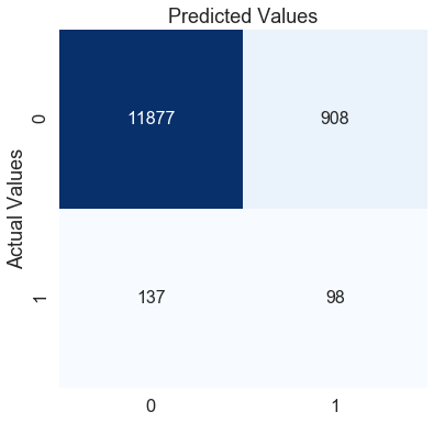
By manually changing the values of the weights, we can improve the f1 score further by approximately 6%. The confusion matrix also shows that from the previous model, we can predict class 0 much better but at the cost of misclassification of our class 1. This depends on the business problem or the error type you want to reduce more. Here, we focused on improving the f1 score, which we could do by tweaking the class weights.

Tips to Improve Scoring Further

• Feature Engineering: We have used only the given independent variables for simplicity. You can try creating new features like frequency-based, interaction-based, grouping, descriptive statistics-based, etc.
• Tuning the threshold: By default, the threshold is 0.5 for all algorithms. You can try different threshold values and find the optimal value by using a grid search or randomised search.
• Using Advanced Algorithms: We have used only logistic regression for this explanation. You can try different advanced bagging and boosting algorithms. Finally, we can also try stacking or blending the multiple algorithms.

Conclusion

I hope this article gave you a good idea of how class weights can help handle a class imbalance problem and how easy it is to implement in Python.

Although we have discussed how class weight works only for logistic regression, the idea remains the same for every other algorithm; it’s just the change of the cost function that each algorithm uses to minimize the error and optimize results for the minority class.

Frequently Asked Questions