Introduction
This is Part-4 of the four-part blog series on Bayesian Decision Theory.
In the previous article, we talked about discriminant functions, classifiers, Decision Surfaces, and Normal density including Univariate as well as Multivariate Normal Distribution. Now, in the final article, we will look at the discriminant functions for normal density under various considerations in Bayesian Decision Theory.
For previous articles, Links are Part-1, Part-2, and Part-3.
Let’s get started,
As discussed in previous article, our discriminant function is given by,
gi(x) = ln p(x|ωi) + ln P(ωi)
As for the normal density p(x|ωi) follows the multivariate normal distribution, so our discriminant function can be written as
gi(x)= -1/2(x-μi)tΣi–1(x-μi) – d/2ln2π – 1/2 ln(|Σi|) +ln(P(wi))
We will now examine this discriminant function in detail by dividing the covariance into different cases.
Case-1 ( Σi = σ2 I )
This case occurs when σij =0 for i!=j i.e, the covariances are zero and the variance of feature i.e σii remains σ2. This implies that the features are statistically independent and each feature has variance σ2. As |Σi| and d/2ln2π term are independent of i and will not change accordingly to the cases, as well as remain unimportant, so they can be ignored.
Substituting our assumption in the normal discriminant function we get,
gi(x) = – ||x – μi||2/2σ2+ ln P(wi)
Where the Euclidean norm is
||x − μi||2 = (x − μi)t(x − μi)
Here we notice that our discriminant function is the sum of two terms, the squared distance from the mean is normalized by the variance and the other term is the log of prior. Our decision favors the prior if x is near the mean.
Stressing more on our equation is can be further expanded as,
gi(x) = − 1/2σ2 [xtx − 2μitx + μitμi] + ln P(ωi)
Here the quadratic term xtx is the same for all i, which could also be ignored. Hence, we arrive at the equivalent linear discriminant functions.
gi(x)= wiT x +wi0
Comparing
wi = 1/σ2 μi
And wi0 = −1/2σ2μitμi + ln P(ωi)
where w0 is the threshold or bias in the ith direction
Such classifiers that use linear discriminant functions are often called linear machines.
We choose the decision surface for any linear machine such that the hyperplane is defined by the equation gi(x)= gj(x) for bi-categorical with the highest posterior probabilities.
Applying the above condition we get,
wt(x − x0) = 0
w = μi − μj
x0 = 1/2(μi + μj) − σ2/ ||μi − μj||2 ln P(wi)/P(ωj)(μi − μj)
The above equation is of a hyperplane through the point x0 and orthogonal to vector w. We can also notice that w = µi −µj, the hyperplane separating the two regions Ri and Rj.
Further, if P(ωi)= P(ωj) the subtractive term in x0 vanishes, and the hyperplane is perpendicular bisector or halfway the means.
Fig. As the priors change, the decision boundary throughout point x0 shifts away from the more common class mean (two-dimensional Gaussian distributions)
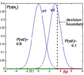
Fig. As the priors change, the decision boundary throughout point x0 shifts away from the more common class mean (one-dimensional Gaussian distributions)
Image Source: link
Case- 2 ( Σi = Σ )
These cases rarely occur, but hold importance when having a transition from case-1 to the more generalized case-3. In this case, the covariance matrix for all of the classes is identical. Even here we can ignore the term d/2ln2π and |Σi|. This eventually leads us to the equation,
gi(x) = −1/2(x − μi)tΣ−1(x − μi) + ln P(ωi)
If the prior probabilities P(wi) are the same for all the classes the decision rule remains that to choose the feature vector x to the class with the nearest mean vector of class c. If the prior probabilities are biased the decision is in favor of the prior more likely class.
The quadratic form (x−µi)tΣ−1(x−µi) can be expanded as we again notice that the term xtΣ−1x can be ignored as it is independent of i. After this term is dropped we get the linear discriminant function.
gi(x) = witx + wi0
wi = Σ−1μi
wi0 =−1/2μitΣ−1μi+ln P(ωi)
As the discriminant function is linear the outcome of decision boundaries are again the hyperplane with the equation,
wt(x − x0) = 0
w = Σ−1(μi −μj)
x0 = 1/2 (μi + μj) − { ln [P(ωi)/P(ωj)]/(μi − μj)tΣ−1(μi − μj) }(μi – μj)
The difference this hyperplane has as compared from the on in case 1 is that it is not orthogonal to the line between the means and also it does not intersect halfway the point between the means if the priors are equal.
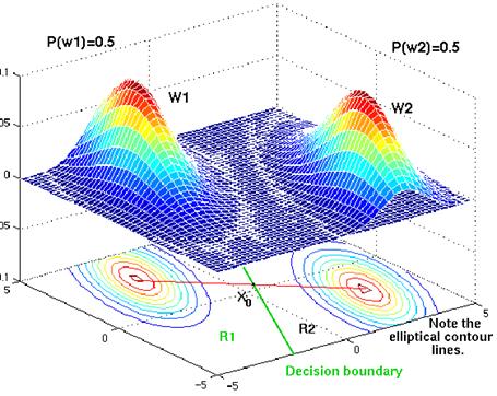
Fig. The contour lines are elliptical in shape because the covariance matrix is not diagonal. However, both densities show the same elliptical shape. The prior probabilities are the same, and so the point x0 lies halfway between the 2 means. The decision boundary is not orthogonal to the red line. Instead, it is tilted so that its points are of equal distance to the contour lines in w1 and those in w2.
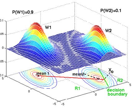
Fig. The contour lines are elliptical, but the prior probabilities are different. Although the decision boundary is a parallel line, it has been shifted away from the more likely class. With sufficient bias, the decision boundary can be shifted so that it no longer lies between the 2 means
Image Source: link
Case- 3 ( Σi = arbitrary )
We now come to the most realistic case of the covariance being different for each class, Now the only term dropped from the discriminant function equation of normal multivariate density is the d/2ln2π.
The resulting discriminant function no more remains linear, as it inherently stays quadratic:
gi(x) = xtWix + witx + wi0
Wi = −1/2 Σi−1
wi = Σi−1μi
wi0 = −1/2μitΣi−1μi − 1/2ln |Σi| + ln P(ωi)
The decision surfaces are hyperquadrics i.e general form of hyperplanes, pairs of hyperplanes, hyperspheres, hyperparaboloids, and more freaky shapes. The extension to the more than two categories is straightforward. Some cool decision boundaries of 2-D and 3-D can be seen below
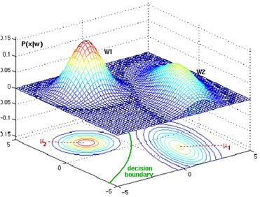
Fig. Two bivariate normals, with completely different covariance matrix, are showing a hyper quadratic decision boundary.
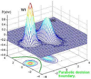
Fig. Example of parabolic decision surface.
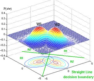
Fig. Example of straight decision surface.
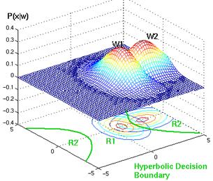
Fig. Example of hyperbolic decision surface.
Image Source: link
This completes our Bayesian Decision Theory in a detailed manner!
Discussion Problems
Problem-1:
Consider a two-class one-feature classification problem with gaussian densities p(x|w1) = N(0, 1) and p(x|w2) = N(1, 2). Assume equal prior probabilities. Now, answer the below questions:
1. Determine the decision boundary.
2. If prior probabilities are changed and P(w1) = 0.6 and P(w2) = 0.4, then calculate the new decision boundary?
Problem-2:
If there are 3n variables and one binary label, how many numbers of parameters are required to represent the naive Bayes classifier?
Problem-3:
In the discriminant functions for the normal density where features are independent and such feature vector has the same variance σ2, then we can easily calculate the determinant Σ by____?
Try to solve the Practice Questions and answer them in the comment section below.
For any further queries feel free to contact me.
End Notes
Thanks for reading!
If you liked this and want to know more, go visit my other articles on Data Science and Machine Learning by clicking on the Link
Please feel free to contact me on Linkedin, Email.
Something not mentioned or want to share your thoughts? Feel free to comment below And I’ll get back to you.
About the author
Chirag Goyal
Currently, I am pursuing my Bachelor of Technology (B.Tech) in Computer Science and Engineering from the Indian Institute of Technology Jodhpur(IITJ). I am very enthusiastic about Machine learning, Deep Learning, and Artificial Intelligence.
The media shown in this article on Bayesian Decision Theory are not owned by Analytics Vidhya and are used at the Author’s discretion.
I am a B.Tech. student (Computer Science major) currently in the pre-final year of my undergrad. My interest lies in the field of Data Science and Machine Learning. I have been pursuing this interest and am eager to work more in these directions. I feel proud to share that I am one of the best students in my class who has a desire to learn many new things in my field.


