What is Supervised Machine Learning?

Machine Learning (ML) allows computers to learn patterns from data and make decisions by themselves. Think of it as teaching machines how to “learn from experience.” We allow the machine to learn the rules from examples rather than hardcoding each one. It is the concept at the center of the AI revolution. In this article, we’ll go over what supervised learning is, its different types, and some of the common algorithms that fall under the supervised learning umbrella.

What is Machine Learning?

Fundamentally, machine learning is the process of identifying patterns in data. The main concept is to create models that perform well when applied to fresh, untested data. ML can be broadly categorised into three areas:

1. Supervised Learning
2. Unsupervised Learning
3. Reinforcement Learning

Simple Example: Students in a Classroom

• In supervised learning, a teacher gives students questions and answers (e.g., “2 + 2 = 4”) and then quizzes them later to check if they remember the pattern.
• In unsupervised learning, students receive a pile of data or articles and group them by topic; they learn without labels by identifying similarities.

Now, let’s try to understand Supervised Machine Learning technically.

What is Supervised Machine Learning?

In supervised learning, the model learns from labelled data by using input-output pairs from a dataset. The mapping between the inputs (also referred to as features or independent variables) and outputs (also referred to as labels or dependent variables) is learned by the model. Making predictions on unknown data using this learned relationship is the aim. The goal is to make predictions on unseen data based on this learned relationship. Supervised learning tasks fall into two main categories:

1. Classification

The output variable in classification is categorical, meaning it falls into a specific group of classes.

Examples:

• Email Spam Detection
  • Input: Email text
  • Output: Spam or Not Spam
• Handwritten Digit Recognition (MNIST)
  • Input: Image of a digit
  • Output: Digit from 0 to 9

2. Regression

The output variable in regression is continuous, meaning it can have any number of values that fall within a specific range.

Examples:

• House Price Prediction
  • Input: Size, location, number of rooms
  • Output: House price (in dollars)
• Stock Price Forecasting
  • Input: Previous prices, volume traded
  • Output: Next day’s closing price

Supervised Learning Workflow 

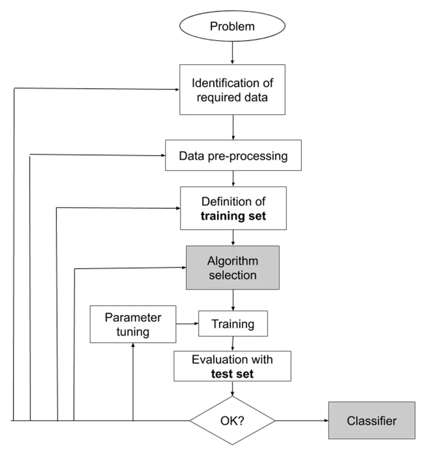
A typical supervised machine learning algorithm follows the workflow below:

1. Data Collection: Collecting labelled data is the first step, which entails collecting both the correct outputs (labels) and the inputs (independent variables or features).
2. Data Preprocessing: Before training, our data must be cleaned and prepared, as real-world data is often disorganized and unstructured. This entails dealing with missing values, normalising scales, encoding text to numbers, and formatting data appropriately.
3. Train-Test Split: To test how well your model generalizes to new data, you need to split the dataset into two parts: one for training the model and another for testing it. Typically, data scientists use around 70–80% of the data for training and reserve the rest for testing or validation. Most people use 80-20 or 70-30 splits.
4. Model Selection: Depending on the type of problem (classification or regression) and the nature of your data, you choose an appropriate machine learning algorithm, like linear regression for predicting numbers, or decision trees for classification tasks.
5. Training: The training data is then used to train the chosen model. The model gains knowledge of the fundamental trends and connections between the input features and the output labels in this step.
6. Evaluation: The unseen test data is used to evaluate the model after it has been trained. Depending on whether it’s a classification or regression task, you assess its performance using metrics like accuracy, precision, recall, RMSE, or F1-score.
7. Prediction: Lastly, the trained model predicts outputs for new, real-world data with unknown results. If it performs well, teams can use it for applications like price forecasting, fraud detection, and recommendation systems.

Common Supervised Machine Learning Algorithms

Let’s now look at some of the most commonly used supervised ML algorithms. Here, we’ll keep things simple and give you an overview of what each algorithm does.

1. Linear Regression

Fundamentally, linear regression determines the optimal straight-line relationship (Y = aX + b) between a continuous target (Y) and input features (X). By minimizing the sum of squared errors between the expected and actual values, it determines the optimal coefficients (a, b). It is computationally efficient for modeling linear trends, such as forecasting home prices based on location or square footage, thanks to this closed-form mathematical solution. When relationships are roughly linear and interpretability is important, their simplicity shines.

2. Logistic Regression

In spite of its name, logistic regression converts linear outputs into probabilities to address binary classification. It squeezes values between 0 and 1, which represent class likelihood, using the sigmoid function (1 / (1 + e⁻ᶻ)) (e.g., “cancer risk: 87%”). At probability thresholds (usually 0.5), decision boundaries appear. Because of its probabilistic basis, it is perfect for medical diagnosis, where comprehension of uncertainty is just as important as making accurate predictions.

3. Decision Trees

Decision trees are a simple machine learning tool used for classification and regression tasks. These user-friendly “if-else” flowcharts use feature thresholds (such as “Income > $50k?”) to divide data hierarchically. Algorithms such as CART optimise information gain (lowering entropy/variance) at each node to distinguish classes or forecast values. Final predictions are produced by terminal leaves. Although they run the risk of overfitting noisy data, their white-box nature aids bankers in explaining loan denials (“Denied due to credit score < 600 and debt ratio > 40%”).

4. Random Forest

An ensemble method that uses random feature samples and data subsets to construct multiple decorrelated decision trees. It uses majority voting to aggregate predictions for classification and averages for regression. For credit risk modeling, where single trees could confuse noise for pattern, it is robust because it reduces variance and overfitting by combining a variety of “weak learners.”

5. Support Vector Machines (SVM)

In high-dimensional space, SVMs determine the best hyperplane to maximally divide classes. To deal with non-linear boundaries, they implicitly map data to higher dimensions using kernel tricks (like RBF). In text/genomic data, where classification is defined solely by key features, the emphasis on “support vectors” (critical boundary cases) provides efficiency.

6. K-nearest Neighbours (KNN)

A lazy, instance-based algorithm that uses the majority vote of its k closest neighbours within feature space to classify points. Similarity is measured by distance metrics (Euclidean/Manhattan), and smoothing is controlled by k. It has no training phase and instantly adjusts to new data, making it ideal for recommender systems that make movie recommendations based on similar user preferences.

7. Naive Bayes

This probabilistic classifier makes the bold assumption that features are conditionally independent given the class to apply Bayes’ theorem. It uses frequency counts to quickly compute posterior probabilities in spite of this “naivety.” Millions of emails are scanned by real-time spam filters because of their O(n) complexity and sparse-data tolerance.

8. Gradient Boosting (XGBoost, LightGBM)

A sequential ensemble in which every new weak learner (tree) fixes the mistakes of its predecessor. By using gradient descent to optimise loss functions (such as squared error), it fits residuals. By adding regularisation and parallel processing, advanced implementations such as XGBoost dominate Kaggle competitions by achieving accuracy on tabular data with intricate interactions.

Real-World Applications

Some of the applications of supervised learning are:

• Healthcare: Supervised learning revolutionises diagnostics. Convolutional Neural Networks (CNNs) classify tumours in MRI scans with above 95% accuracy, while regression models predict patient lifespans or drug efficacy. For example, Google’s LYNA detects breast cancer metastases faster than human pathologists, enabling earlier interventions.
• Finance: Classifiers are used by banks for credit scoring and fraud detection, analysing transaction patterns to identify irregularities. Regression models use historical market data to predict loan defaults or stock trends. By automating document analysis, JPMorgan’s COIN platform saves 360,000 labour hours a year.
• Retail & Marketing: A combination of techniques called collaborative filtering is used by Amazon’s recommendation engines to make product recommendations, increasing sales by 35%. Regression forecasts demand spikes for inventory optimization, while classifiers use purchase history to predict the loss of customers.
• Autonomous Systems: Self-driving cars rely on real-time object classifiers like YOLO (“You Only Look Once”) to identify pedestrians and traffic signs. Regression models calculate collision risks and steering angles, enabling safe navigation in dynamic environments.

Critical Challenges & Mitigations

Challenge 1: Overfitting vs. Underfitting

Overfitting occurs when models memorise training noise, failing on new data. Solutions include regularisation (penalising complexity), cross-validation, and ensemble methods. Underfitting arises from oversimplification; fixes involve feature engineering or advanced algorithms. Balancing both optimises generalisation.

Challenge 2: Data Quality & Bias

Biased data produces discriminatory models, especially in the sampling process(e.g., gender-biased hiring tools). Mitigations include synthetic data generation (SMOTE), fairness-aware algorithms, and diverse data sourcing. Rigorous audits and “model cards” documenting limitations enhance transparency and accountability.

Challenge 3: The “Curse of Dimensionality”

High-dimensional data (10k features) requires an exponentially larger number of samples to avoid sparsity. Dimensionality reduction techniques like PCA (Principal Component Analysis), LDA (Linear Discriminant Analysis) take these sparse features and reduce them while retaining the informative information, allowing analysts to make better evict decisions based on smaller groups, which improves efficiency and accuracy. 

Conclusion

Supervised Machine Learning (SML) bridges the gap between raw data and intelligent action. By learning from labelled examples enables systems to make accurate predictions and informed decisions, from filtering spam and detecting fraud to forecasting markets and aiding healthcare. In this guide, we covered the foundational workflow, key types (classification and regression), and essential algorithms that power real-world applications. SML continues to shape the backbone of many technologies we rely on every day, often without even realising it.