Crash Course to Crack Machine Learning Interview – Part 1: Bias vs Variance

Preparing for machine learning interviews? One of the most fundamental concepts you’ll encounter is the bias-variance tradeoff. This isn’t just theoretical knowledge – it’s the cornerstone of understanding why models succeed or fail in real-world applications. Whether you’re interviewing at Google, Netflix, or a startup, mastering this concept will help you stand out from other candidates.

In this comprehensive guide, we’ll break down everything you need to know about bias and variance, complete with the 10 most common interview questions and practical examples you can implement right away.

Understanding the Core Concepts

When an interviewer asks you about bias and variance, they’re not just testing your ability to recite definitions from a textbook. They want to see if you understand how these concepts translate into real-world model-building decisions. Let’s start with the foundational question that sets the stage for everything else.

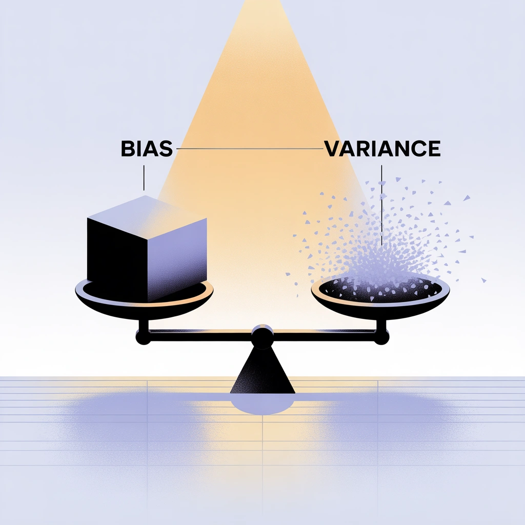
What exactly is bias in machine learning? Bias represents the systematic error that occurs when your model makes simplifying assumptions about the data. In machine learning terms, bias measures how far off your model’s predictions are from the true values, on average, across different possible training sets.

Consider a real-world scenario where you’re trying to predict house prices. If you use a simple linear regression model that only considers the square footage of a house, you’re introducing bias into your system. This model assumes a perfectly linear relationship between house prices and size, while ignoring crucial factors such as location, neighborhood quality, property age, and local market conditions. Your model might consistently undervalue houses in premium neighbourhoods and overvalue houses in less desirable areas—this systematic error is bias.

Variance tells a completely different story. While bias is about being systematically wrong, variance is about being inconsistent. Variance measures how much your model’s predictions change when you train it on slightly different datasets. 

Going back to our house price prediction example, imagine you’re using a very deep decision tree instead of linear regression. This complex model might perform brilliantly on your training data, capturing every nuance and detail. But here’s the problem: if you collect a new set of training data from the same market, your decision tree might look completely different. This sensitivity to training data variations is variance.

Navigating the Bias-Variance Tradeoff

The bias-variance tradeoff represents one of the most elegant and fundamental insights in machine learning. It’s not just a theoretical concept—it’s a practical framework that guides every major decision you make when building predictive models.

Why can’t we just minimize both bias and variance simultaneously? This is where the “tradeoff” part becomes crucial. In most real-world scenarios, reducing bias requires making your model more complex, which inevitably increases variance. Conversely, reducing variance typically requires simplifying your model, which increases bias. It’s like trying to be both extremely detailed and highly consistent in your explanations—the more specific and detailed you get, the more likely you are to say different things in different situations.

How does this play out with different algorithms? Linear regression algorithms like ordinary least squares tend to have high bias but low variance. They make strong assumptions about the relationship between features and targets (assuming it’s linear), but they produce consistent results across different training sets. On the other hand, algorithms like decision trees or k-nearest neighbors can have low bias but high variance—they can model complex, non-linear relationships but are sensitive to changes in training data.

Consider the k-nearest neighbour algorithm as a perfect example of how you can control this tradeoff. When k=1 (using only the closest neighbour for predictions), you have very low bias because the model doesn’t make assumptions about the underlying function. However, variance is extremely high because your prediction depends entirely on which single point happens to be closest. As you increase k, you’re averaging over more neighbours, which reduces variance but increases bias because you’re now assuming that the function is relatively smooth in local regions.

Detecting the Telltale Signs: Overfitting vs Underfitting in Practice

Being able to diagnose whether your model suffers from high bias or high variance is a crucial skill that interviewers love to test. The good news is that there are clear, practical ways to identify these issues in your models.

Underfitting occurs when your model has high bias. The symptoms are unmistakable: poor performance on both training and validation data, with training and validation errors that are similar but both unacceptably high. It’s like studying for an exam by only reading the chapter summaries—you’ll perform poorly on both practice tests and the real exam because you haven’t captured enough detail. In practical terms, if your linear regression model achieves only 60% accuracy on both training and test data when predicting whether emails are spam, you’re likely dealing with underfitting. The model isn’t complex enough to capture the nuanced patterns that distinguish spam from legitimate emails. You might notice that the model treats all emails with certain keywords the same way, regardless of context.

Overfitting manifests as high variance. The classic symptoms include excellent performance on training data but significantly worse performance on validation or test data. Your model has essentially memorized the training examples rather than learning generalizable patterns. It’s like a student who memorizes all the practice problems but can’t solve new problems because they never learned the underlying principles. A telltale sign of overfitting is when your training accuracy reaches 95% but your validation accuracy hovers around 70%. 

Reducing Bias and Variance in Real Models

To address high bias (underfitting), increase model complexity by using more sophisticated algorithms like neural networks, engineering more informative features, adding polynomial terms, or removing excessive regularization. Collecting more diverse training data can also help the model capture underlying patterns.

For high variance (overfitting), apply regularization techniques like L1/L2 to constrain the model. Use cross-validation to obtain reliable performance estimates and prevent overfitting to specific data splits. Ensemble methods such as Random Forests or Gradient Boosting are highly effective, as they combine multiple models to average out errors and reduce variance. Additionally, more training data generally helps lower variance by making the model less sensitive to noise, though it doesn’t fix inherent bias.

Common Interview Questions on Bias and Variance 

Here are some of the commonly asked interview questions on Bias and Variance:

Q1. What do you understand by the terms bias and variance in machine learning?

A. Bias represents the systematic error introduced when your model makes oversimplified assumptions about the data. Think of it as consistently missing the target in the same direction – like a rifle that’s improperly calibrated and always shoots slightly to the left. Variance, on the other hand, measures how much your model’s predictions change when trained on different datasets. It’s like having inconsistent aim – sometimes hitting left, sometimes right, but scattered around the target.

Follow-up: “Can you give a real-world example of each?”

Q2. Explain the bias-variance tradeoff.

A. The bias-variance tradeoff is the fundamental principle that you cannot simultaneously minimize both bias and variance. As you make your model more complex to reduce bias (better fit to training data), you inevitably increase variance (sensitivity to training data changes). The goal is finding the optimal balance where total error is minimised. This tradeoff is crucial because it guides every major decision in model selection, from choosing algorithms to tuning hyperparameters.

Follow-up: “How do you find the optimal point in practice?”

Q3. How do bias and variance contribute to the overall prediction error?

A. The total expected error of any machine learning model can be mathematically decomposed into three components: Total Error = Bias² + Variance + Irreducible Error. Bias squared represents systematic errors from model assumptions, variance captures the model’s sensitivity to training data variations, and irreducible error is the inherent noise in the data that no model can eliminate. Understanding this decomposition helps you identify which component to focus on when improving model performance.

Follow-up: “What is irreducible error, and can it be minimized?”

Q4. How would you detect if your model has high bias or high variance?

A. High bias manifests as poor performance on both training and test datasets, with similar error levels on both. Your model consistently underperforms because it’s too simple to capture the underlying patterns. High variance shows excellent training performance but poor test performance – a large gap between training and validation errors. You can diagnose these issues using learning curves, cross-validation results, and comparing training versus validation metrics.

Follow-up: “What do you do if you detect both high bias and high variance?”

Q5. Which machine learning algorithms are prone to high bias vs high variance?

A. High bias algorithms include linear regression, logistic regression, and Naive Bayes – they make strong assumptions about data relationships. High variance algorithms include deep decision trees, k-nearest neighbors with low k values, and complex neural networks – they can model intricate patterns but are sensitive to training data changes. Balanced algorithms like Support Vector Machines and Random Forest (through ensemble averaging) manage both bias and variance more effectively.

Follow-up: “Why does k in KNN affect the bias-variance tradeoff?”

Q6. How does model complexity affect the bias-variance tradeoff?

A. Simple models (like linear regression) have high bias. They make restrictive assumptions, but low variance because they’re stable across different training sets. Complex models (like deep neural networks) have low bias because they can approximate any function, but high variance because they’re sensitive to training data specifics. The relationship typically follows a U-shaped curve where optimal complexity minimizes the sum of bias and variance.

Follow-up: “How does the training data size affect this relationship?”

Q7. What techniques can you use to reduce high bias in a model?

A. To combat high bias, you need to increase your model’s capacity to learn complex patterns. Use more sophisticated algorithms (switch from linear to polynomial regression), add more relevant features through feature engineering, reduce regularization constraints that oversimplify the model, or collect more diverse training data that better represents the problem’s complexity. Sometimes the solution is recognizing that your feature set doesn’t adequately capture the problem’s nuances.

Follow-up: “When would you choose a biased model over an unbiased one?”

Q8. What methods would you employ to reduce high variance without increasing bias?

A. Regularization techniques like L1 (Lasso) and L2 (Ridge) add penalties to prevent overfitting. Cross-validation provides more reliable performance estimates by testing on multiple data subsets. Ensemble methods like Random Forest and bagging combine multiple models to reduce individual model variance. Early stopping prevents neural networks from overfitting, and feature selection removes noisy variables that contribute to variance.

Follow-up: “How do ensemble methods like Random Forest address variance?”

Q9. How do you use learning curves to diagnose bias and variance issues?

A. Learning curves plot model performance against training set size or model complexity. High bias appears as training and validation errors that are both high and converge to similar values – your model is consistently underperforming. High variance shows up as a large gap between low training error and high validation error that persists even with more data. Optimal models show converging curves at low error levels with a minimal gap between training and validation performance.

Follow-up: “What does it mean if learning curves converge versus diverge?”

Q10. Explain how regularization techniques help manage the bias-variance tradeoff.

A. Regularization adds penalty terms to the model’s cost function to control complexity. L1 regularization (Lasso) can drive some coefficients to zero, effectively performing feature selection, which increases bias slightly but reduces variance significantly. L2 regularization (Ridge) shrinks coefficients toward zero without eliminating them, smoothing the model’s behavior and reducing sensitivity to training data variations. The regularization parameter lets you tune the bias-variance tradeoff – higher regularization increases bias but decreases variance.

Follow-up: “How do you choose the right regularization parameter?”

Read more: Get the most out of Bias-Variance Tradeoff

Conclusion

Mastering bias and variance concepts is about developing the intuition and practical skills needed to build models that work reliably in production environments. The concepts we’ve explored form the foundation for understanding why some models generalize well while others don’t, why ensemble methods are so effective, and how to diagnose and fix common modeling problems.

The key insight is that bias and variance represent complementary perspectives on model error, and managing their tradeoff is central to successful machine learning practice. By understanding how different algorithms, model complexities, and training strategies affect this tradeoff, you’ll be equipped to make informed decisions about model selection, hyperparameter tuning, and performance optimization.

Frequently Asked Questions