How to Run your ML Notebook on Databricks?

Databricks is one of the leading platforms for building and executing machine learning notebooks at scale. It combines Apache Spark capabilities with a notebook-preferring interface, experiment tracking, and integrated data tooling. Here in this article, I’ll guide you through the process of hosting your ML notebook in Databricks step by step. Databricks offers several plans, but for this article, I’ll be using the Free Edition, as it is suitable for learning, testing, and small projects. 

Understanding Databricks Plans

Before we get started, let’s just quickly go through all the Databricks plans that are available. 

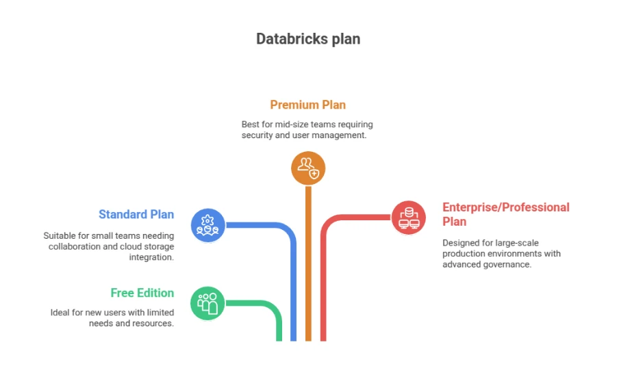
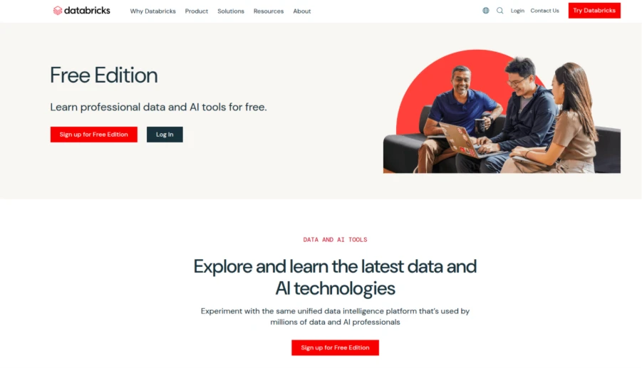
1. Free Edition 

The Free Edition (previously Community Edition) is the simplest way to begin. 
You can sign up at databricks.com/learn/free-edition. 

It has: 

• A single-user workspace 
• Access to a small compute cluster 
• Support for Python, SQL, and Scala 
• MLflow integration for experiment tracking 

It’s totally free and is in a hosted environment. The biggest drawbacks are that clusters timeout after an idle time, resources are limited, and some enterprise capabilities are turned off. Nonetheless, it’s ideal for new users or users trying Databricks for the first time. 

2. Standard Plan 

The Standard plan is ideal for small teams. 

It provides additional workspace collaboration, larger compute clusters, and integration with your own cloud storage (such as AWS or Azure Data Lake). 

This level allows you to connect to your data warehouse and manually scale up your compute when required. 

3. Premium Plan 

The Premium plan introduces security features, role-based access control (RBAC), and compliance. 

It’s typical of mid-size teams that require user management, audit logging, and integration with business identity systems. 

4. Enterprise / Professional Plan 

The Enterprise or Professional plan (depending on your cloud provider) includes all that the Premium plan has, plus more advanced governance capabilities such as Unity Catalog, Delta Live Tables, jobs scheduled automatically, and autoscaling. 

This is generally utilized in production environments with multiple teams operating workloads at scale. For this tutorial, I’ll be using the Databricks Free Edition. 

Hands-on

You can use it to try out Databricks for free and see how it works. 

Here’s how you can follow along. 

Step 1: Sign Up for Databricks Free Edition 

1. Visit https://www.databricks.com/learn/free-edition 

2. Sign up with your email, Google, or Microsoft account. 

3. After you sign in, Databricks will automatically create a workspace for you. 

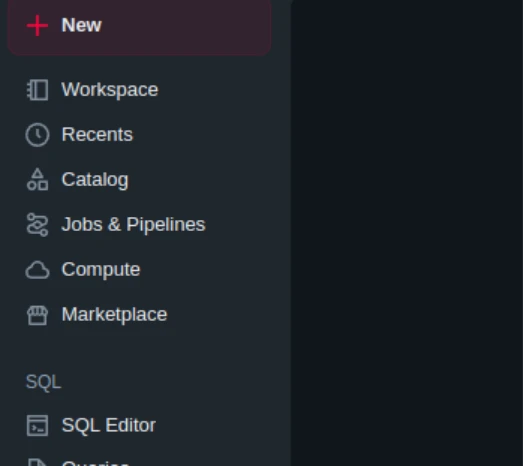
The dashboard that you are looking at is your command center. You can control notebooks, clusters, and data all from here. 

No local installation is required. 

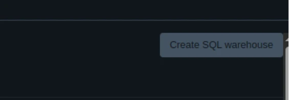
Step 2: Create a Compute Cluster 

Databricks executes code against a cluster, a managed compute environment. You require one to run your notebook. 

1. In the sidebar, navigate to Compute. 

2. Click Create Compute (or Create Cluster). 

3. Name your cluster. 

4. Choose the default runtime (ideally Databricks Runtime for Machine Learning). 

5. Click Create and wait for it to become Running. 

When the status is Running, you’re ready to mount your notebook. 

In the Free Edition, clusters can automatically shut down after inactivity. You can restart them whenever you want. 

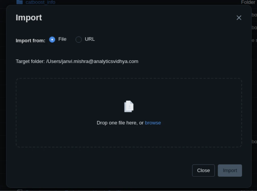
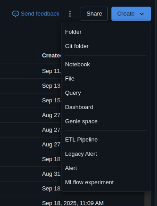
Step 3: Import or Create a Notebook 

You can use your own ML notebook or create a new one from scratch. 

To import a notebook: 

1. Go to Workspace. 
2. Select the dropdown beside your folder → Import → File. 

3. Upload your .ipynb or .py file. 

To create a new one: 

• Click on Create → Notebook. 

After creating, bind the notebook to your running cluster (search for the dropdown at the top). 

Step 4: Install Dependencies 

If your notebook depends on libraries such as scikit-learn, pandas, or xgboost, install them within the notebook. 

Use: 

%pip install scikit-learn pandas xgboost matplotlib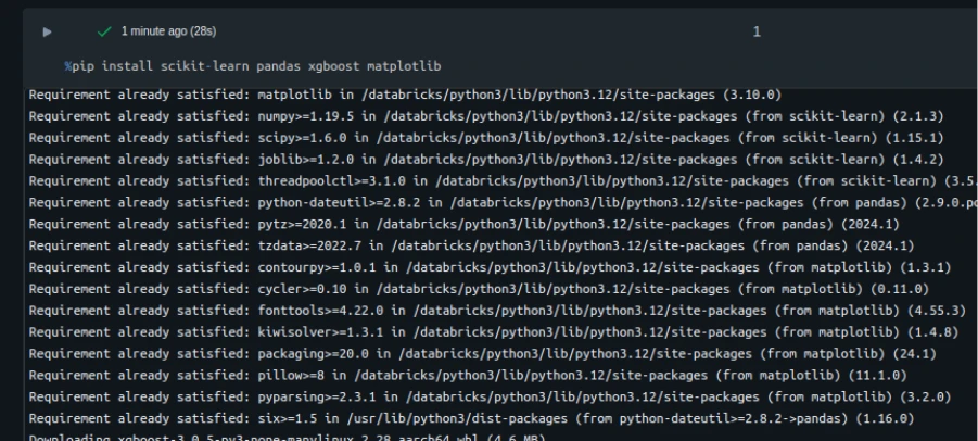 

Databricks might restart the environment after the install; that’s okay.  

Note: You may need to restart the kernel using %restart_python or dbutils.library.restartPython() to use updated packages. 

You can install from a requirements.txt file too: 

%pip install -r requirements.txt 

To verify the setup: 

import sklearn, sys 
print(sys.version) 
print(sklearn.__version__) 

Step 5: Run the Notebook 

You can now execute your code. 

Each cell runs on the Databricks cluster. 

• Press Shift + Enter to run a single cell. 
• Press Run All to run the whole notebook. 

You will get the outputs similarly to those in Jupyter. 

If your notebook has large data operations, Databricks processes them via Spark automatically, even in the free plan. 

You can monitor resource usage and job progress in the Spark UI (available under the cluster details). 

Step 6: Coding in Databricks 

Now that your cluster and environment are set up, let’s learn how you can write and run an ML notebook in Databricks. 

We will go through a full example, the NPS Regression Tutorial, which uses regression modeling to predict customer satisfaction (NPS score). 

1: Load and Inspect Data 

Import your CSV file into your workspace and load it with pandas: 

from pathlib import Path 
import pandas as pd 
 
DATA_PATH = Path("/Workspace/Users/[email protected]/nps_data_with_missing.csv") 
df = pd.read_csv(DATA_PATH) 
df.head()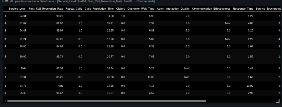

Inspect the data: 

df.info()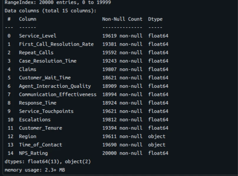 

df.describe().T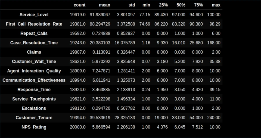 

2: Train/Test Split 

from sklearn.model_selection import train_test_split 
 
TARGET = "NPS_Rating" 
train_df, test_df = train_test_split(df, test_size=0.2, random_state=42) 

train_df.shape, test_df.shape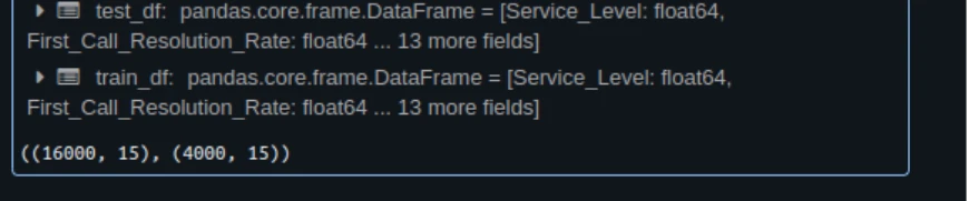

3: Quick EDA 

import matplotlib.pyplot as plt 
import seaborn as sns 
 
sns.histplot(train_df["NPS_Rating"], bins=10, kde=True) 
plt.title("Distribution of NPS Ratings") 
plt.show() 

4: Data Preparation with Pipelines 

from sklearn.pipeline import Pipeline 
from sklearn.compose import ColumnTransformer 
from sklearn.impute import KNNImputer, SimpleImputer 
from sklearn.preprocessing import StandardScaler, OneHotEncoder 
 
num_cols = train_df.select_dtypes("number").columns.drop("NPS_Rating").tolist() 
cat_cols = train_df.select_dtypes(include=["object", "category"]).columns.tolist() 
 
numeric_pipeline = Pipeline([ 
   ("imputer", KNNImputer(n_neighbors=5)), 
   ("scaler", StandardScaler()) 
]) 
 
categorical_pipeline = Pipeline([ 
   ("imputer", SimpleImputer(strategy="constant", fill_value="Unknown")), 
   ("ohe", OneHotEncoder(handle_unknown="ignore", sparse_output=False)) 
]) 
 
preprocess = ColumnTransformer([ 
   ("num", numeric_pipeline, num_cols), 
   ("cat", categorical_pipeline, cat_cols) 
]) 

5: Train the Model 

from sklearn.linear_model import LinearRegression 
from sklearn.metrics import r2_score, mean_squared_error 
 
lin_pipeline = Pipeline([ 
  ("preprocess", preprocess), 
   ("model", LinearRegression()) 
]) 
 
lin_pipeline.fit(train_df.drop(columns=["NPS_Rating"]), train_df["NPS_Rating"]) 

6: Evaluate Model Performance 

y_pred = lin_pipeline.predict(test_df.drop(columns=["NPS_Rating"])) 
 
r2 = r2_score(test_df["NPS_Rating"], y_pred) 
rmse = mean_squared_error(test_df["NPS_Rating"], y_pred, squared=False) 
 
print(f"Test R2: {r2:.4f}") 
print(f"Test RMSE: {rmse:.4f}")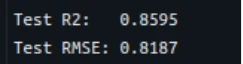 

7: Visualize Predictions 

plt.scatter(test_df["NPS_Rating"], y_pred, alpha=0.7) 
plt.xlabel("Actual NPS") 
plt.ylabel("Predicted NPS") 
plt.title("Predicted vs Actual NPS Scores") 
plt.show() 

8: Feature Importance 

ohe = lin_pipeline.named_steps["preprocess"].named_transformers_["cat"].named_steps["ohe"] 
feature_names = num_cols + ohe.get_feature_names_out(cat_cols).tolist() 
 
coefs = lin_pipeline.named_steps["model"].coef_.ravel() 
 
import pandas as pd 
imp_df = pd.DataFrame({"feature": feature_names, "coefficient": coefs}).sort_values("coefficient", ascending=False) 
imp_df.head(10)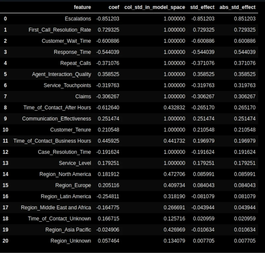 

Visualize: 

top = imp_df.head(15) 
plt.barh(top["feature"][::-1], top["coefficient"][::-1]) 
plt.xlabel("Coefficient") 
plt.title("Top Features Influencing NPS") 
plt.tight_layout() 
plt.show()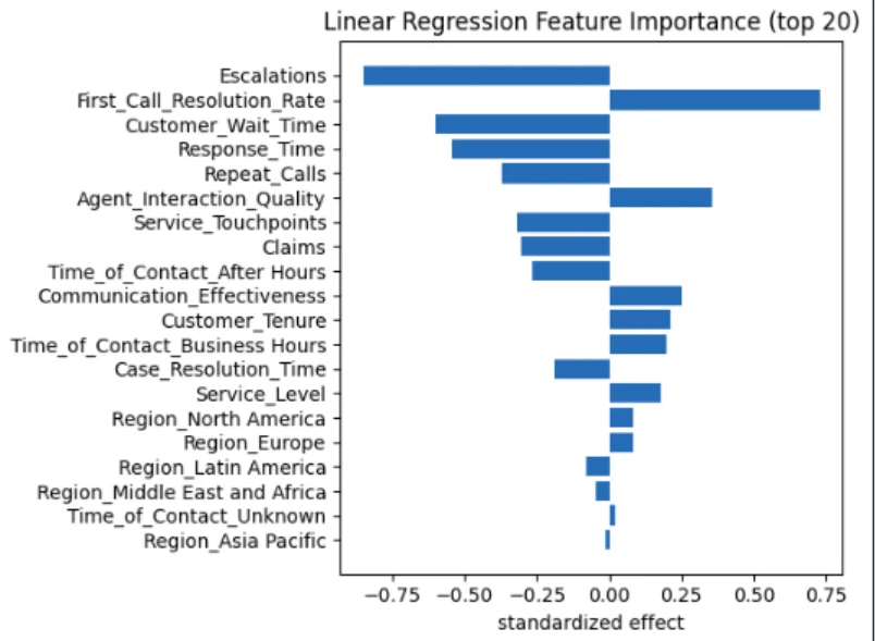 

Step 7: Save and Share Your Work 

Databricks notebooks automatically save to your workspace.

You can export them to share or save them for a backup. 

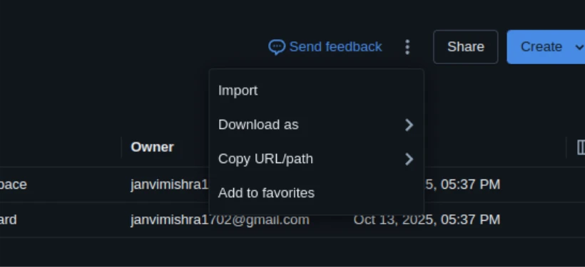
• Navigate to File → Click on the three dots and then click on Download  
• Select .ipynb, .dbc, or .html 

You can also link your GitHub repository under Repos for version control. 

Things to Know About Free Edition

Free Edition is wonderful, but don’t forget the following: 

• Clusters shut down after an idle time (approximately 2 hours). 
• Storage capacity is limited. 
• Certain enterprise capabilities are unavailable (such as Delta Live Tables and job scheduling). 
• It’s not for production workloads. 

Nevertheless, it’s a perfect environment to learn ML, try Spark, and test models.

Conclusion

Databricks makes cloud execution of ML notebooks easy. It requires no local install or infrastructure. You can begin with the Free Edition, develop and test your models, and upgrade to a paid plan later if you require additional power or collaboration features. Whether you are a student, data scientist, or ML engineer, Databricks provides a seamless journey from prototype to production. 

If you have not used it before, go to this website and begin running your own ML notebooks today. 

Frequently Asked Questions