Getting Started with XGBoost: A Beginner-Friendly Tutorial

Among all the tools that a data scientist has, it is difficult to find one that has received a reputation as an effective and trustworthy tool like XGBoost. It was even mentioned in the winning solution of machine learning competitions on a site such as Kaggle, which you have probably visited. This isn’t by accident. The XGBoost algorithm is a champion with regard to performance on structured data. This tutorial is the start of what you need to know about XGBoost, and it dissects its functionality and follows a real-life XGBoost Python tutorial.

We are going to see what is so special in the implementation of this gradient boosting. We are also going to examine an XGBoost vs. Random Forest comparison to see where it fits in the ensemble model world. At the end, you will have a clear understanding of how to apply this amazing algorithm to your own projects.

What is XGBoost and Why Should You Use It?

Essentially, XGBoost, the name of which is shortened from eXtreme Gradient Boosting, is an ensemble learning technique. Consider it as the creation of a team of specialized employees rather than depending on a generalist. It uses numerous simple models, generally decision trees, to form a single very accurate and robust predictive model. The errors made by each new tree it adds to the team cause the corresponding model to improve with each new addition.

Why XGBoost?

So why then is XGBoost so popular? The answer is its list of strengths that is so impressive.

• Exceptional Performance: It always provides the highest quality results, particularly in tabular data, which is usually present in business problems.
• Speed and Efficiency: The library is a well-oiled machine. It employs techniques such as parallel processing to learn models in a short time, even when working with huge amounts of data.
• Inbuilt Checks and Balances: A typical aspect of machine learning is overfitting, wherein the model learns too well the training data and is unable to work on new data. XGBoost has regularization methods that serve as a safety net to preclude this.
• Deals with Sloppy Data: Data in the real world is not ideal. XGBoost has an inbuilt capability to handle missing values and will save you the tedious preprocessing phase.
• Versatility: XGBoost is able to work on both a classification problem (such as fraud detection) and a regression task (such as house price prediction).

Of course, no tool is perfect. The XGBoost power is associated with increased complexity. It is not as transparent as a simple linear model, but it is definitely less of a black box than a deep neural network. A single experiment discovered that XGBoost provided a minor accuracy benefit over logistic regression (98% common sense over 97%). This is because it needed ten times as much time to think about and clarify. It is important to know when that additional increase in performance is worth the effort of substituting.

Also Read: Top 10 Machine Learning Algorithms in 2026

How Boosting Works: A Team of Learners

In order to fully appreciate the XGBoost, it is worthwhile to have some concept of boosting. It is another philosophy, as opposed to other ensemble techniques such as bagging, that is applied by the random forests.

Suppose you are presented with two techniques for solving a complicated problem with the help of a group of people.

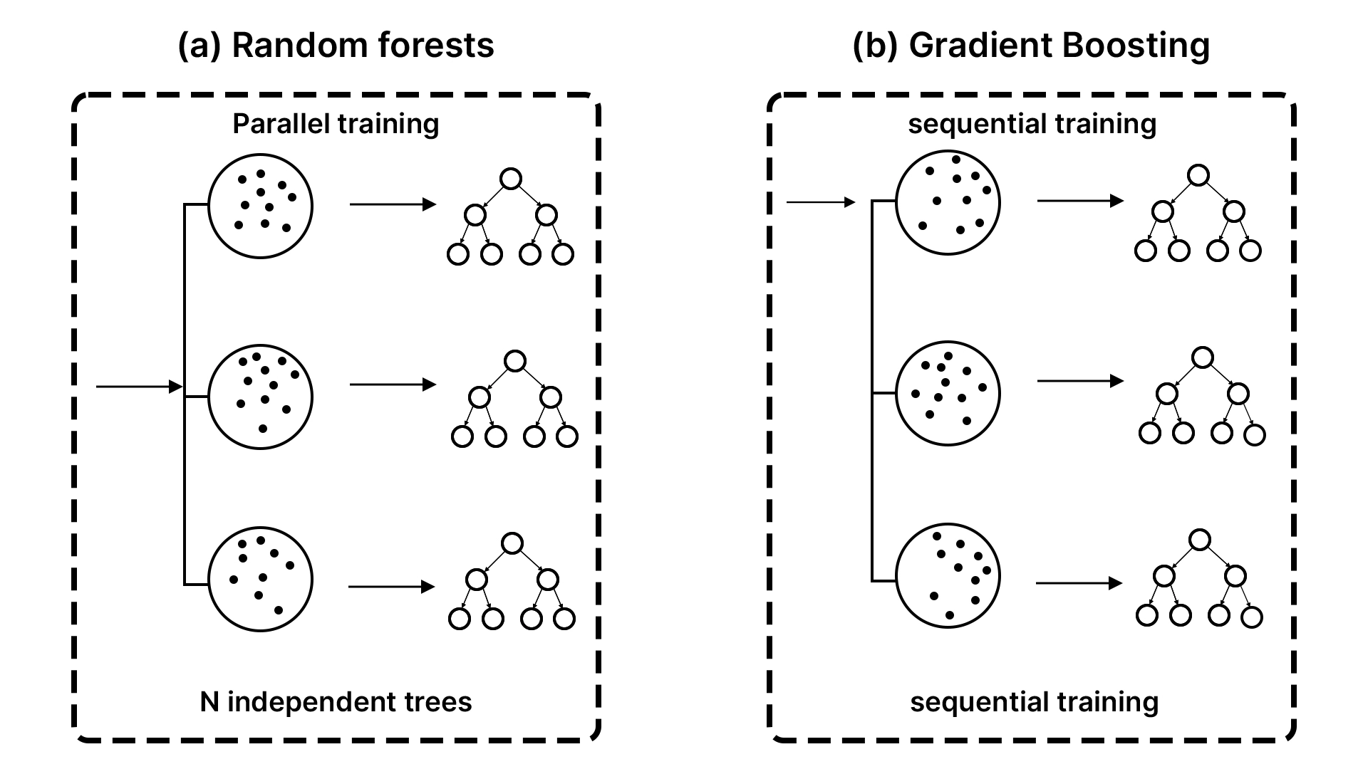
1. Bagging (The Committee Approach): You award a problem to 100 individuals, get them all to work individually, and then majority vote on the final solution. This is the way Random Forest works. It constructs numerous trees on the various random samples of the data and averages the votes.
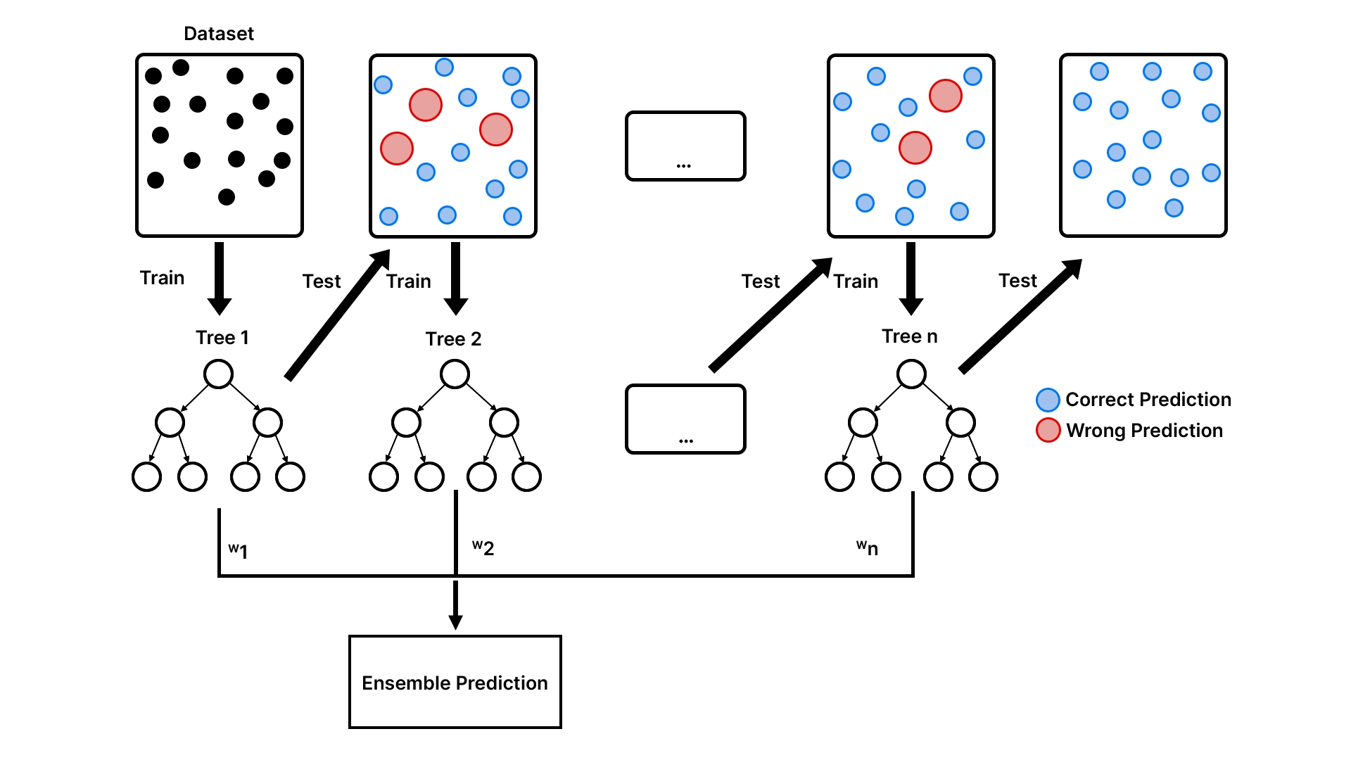
2. Boosting (The Relay Race Approach): You hand the problem over to the initial individual. They work out a resolution but commit some errors. The second person, then, will only look at the errors and attempt to rectify them. The third person corrects the errors of the second person and so forth.

XGBoost is based on the relay race strategy. At a time, the new decision trees are concerned with the data points that the old trees missed. Technically, every new tree has been trained to forecast the errors (also known as residuals) of the existing ensemble. The team becomes resilient as it becomes more precise as time passes, and the inclusion of a model rectifies past mistakes. It is the magic of gradient boosting, which is performed in a sequential and error-correcting way.

All the trees of the process are weak learners, simple shallow trees, which may or may not be any better than guessing. However, when hundreds or thousands of these poor learners are put together in a chain, the resulting model is a powerhouse and a very specific predictor.

How XGBoost Builds Smarter, More Accurate Trees

Decision trees are the fundamental building blocks; therefore, the way that XGBoost expands them has a major influence on its performance. Contrary to other algorithms, which fill out trees with a single branch and then examine the other, XGBoost builds a tree at each level. The given strategy usually gives a better-balanced tree, and optimization becomes more effective.

XGBoost gets its gradient component due to the manner in which splits are selected. At every step, the algorithm considers the degree to which a possible split can decrease the total error of the model and chooses the split that offers the most beneficial way. It is due to this error-sensitive process that XGBoost can effectively learn highly intricate patterns.

In order to minimize overfitting, XGBoost defaults to keeping trees comparatively shallow and uses a learning rate, also referred to as shrinkage. In the learning rate, the input of every new tree is reduced, which forces the model to get better with time. The smaller the learning rates tend to be, the more likely the trees are to create generalisation to the unseen data.

How XGBoost Controls Speed, Scale, and Hardware Efficiency

The parameter of XGBoost also enables you to regulate the development of trees with the help of the tree-method parameter. The simplest option is the histogram-based option, hist, which discretizes feature values and constructs trees based upon the discretized feature values. This is fast and resource-efficient in terms of CPU training. On very large data sets, one can use an alternative approximate technique, approx, but this is less frequently used in current workflows. In cases where a compatible GPU exists, gpuhist uses the same histogram strategy on the GPU and can aid in training time by a wide margin.

hist is, in most instances, a powerful default. Training speed is important, and GPU_hist should be used when GPU acceleration is present, and reserve should be used when specialized large-scale experiments are required.

XGBoost vs. Random Forest vs. Logistic Regression

It is also a good idea to compare XGBoost to the rest of the popular models.

• XGBoost vs. Random Forest (The Relay Race vs. The Committee): XGBoost is also sensitive to the sequence in which the trees are built, as we discussed, thus it is also more right in some situations when it is tuned accordingly. Random Forest produces independent and parallel trees, that imply that it is very stable and less prone to overfitting. XGBoost performs better than the options in most situations where the optimal performance is required, and parameters can be set. Random Forest is also a quite good model to be used in case you need a stable and powerful model that requires minimum efforts.
• XGBoost vs. Logistic Regression (The Power Tool vs. The Swiss Army Knife): Logistic Regression is a simple yet fast and quite easy to interpret linear model. It is used to mark classes in a straight line. It is miraculously working and can be explained easily depending on its verdicts in the situation where your data is linearly separable. The XGBoost is a non-linear model that is quite complex. It can identify complicated patterns and interactions within the data that the Logistic Regression would not have at all. Logistic Regression is used in preference to interpretation. XGBoost is superior to use in the event that one wants to possess predictive accuracy on a difficult issue.

A Practical XGBoost Python Tutorial

We understood the theory, but now it is high time we rolled up our sleeves and went to work. To develop an XGBoost model, we shall utilise the Breast Cancer Wisconsin data that has been utilised to form a benchmark in binary classification. We would like to know whether a tumor is malignant or not in accordance with the measurements of the cells.

1. Loading and Preparing the Data

First of all, we shall feed scikit-learn using our dataset and split it into the training and testing sets. This provides us with the possibility to test the model on one of the sides of the data and the functionality of the model on the other side, which is unknown.

import numpy as np 
import pandas as pd 
import matplotlib.pyplot as plt 
from sklearn.datasets import load_breast_cancer 
from sklearn.model_selection import train_test_split 
from sklearn.metrics import accuracy_score, confusion_matrix, ConfusionMatrixDisplay  

# Load the dataset 
data = load_breast_cancer() 
X = data.data 
y = data.target  

# Split data into 80% training and 20% testing 
# We use stratify=y to ensure the class proportions are the same in train and test sets 
X_train, X_test, y_train, y_test = train_test_split( 
   X, y, test_size=0.2, random_state=42, stratify=y 
) 
 
print(f"Training samples: {X_train.shape[0]}") 
print(f"Test samples: {X_test.shape[0]}")

Output:

Training samples: 455
Test samples:     114

This will give 455 training samples and 114 testing samples. The best things about tree-based models like the XGBoost are that they do not require feature scaling.

DMatrix

NumPy arrays or pandas DataFrames are used directly by most beginners (there is nothing wrong with this). However, internally, the XGBoost has a data structure of its own, namely DMatrix, which is optimized. It is memory efficient and fast, and it has missing values and advanced training.

You usually see DMatrix in the “native” XGBoost API (xgb.train):

import xgboost as xgb 

dtrain = xgb.DMatrix(X_train, label=y_train) 
dtest = xgb.DMatrix(X_test, label=y_test)  

params = { 
"objective": "binary:logistic", 
"eval_metric": "logloss", 
"max_depth": 3, 
"eta": 0.05, # eta = learning_rate in native API 
"subsample": 0.9, 
"colsample_bytree": 0.9 
}  

bst = xgb.train( 
params, 
dtrain, 
num_boost_round=500, 
evals=[(dtest, "test")] 
) 

pred_prob = bst.predict(dtest) 

Output:

[0]   test-logloss:0.61964
[1]   test-logloss:0.58421
[2]   test-logloss:0.55229
[3]   test-logloss:0.52098
[4]   test-logloss:0.49499
[5]   test-logloss:0.46955
[6]   test-logloss:0.44798
[7]   test-logloss:0.42631
[8]   test-logloss:0.40620
[9]   test-logloss:0.38959
[10]  test-logloss:0.37333
[11]  test-logloss:0.35676

2. Training a Basic XGBoost Classifier

At this point, we will be training the first model with the scikit-learn-compatible API of XGBoost.

import xgboost as xgb 

# Initialize the XGBoost classifier 
model = xgb.XGBClassifier(use_label_encoder=False, eval_metric='logloss', random_state=42)  

# Train the model 
model.fit(X_train, y_train) 

# Make predictions on the test set 
y_pred = model.predict(X_test)  

# Evaluate the accuracy 
accuracy = accuracy_score(y_test, y_pred) 
print(f"Test Accuracy: {accuracy*100:.2f}%") 

Output:

Test Accuracy: 95.61%

In default conditions, our model is greater than 95 percent accurate. That’s a strong start. Accuracy, however, does not encompass the whole picture, especially in the medical field. This is because mistakes do not have the same result.

Early Stopping

One of the simplest methods used to avoid overfitting in XGBoost is early stopping. You would not guess the number of trees (n_estimators) you require. Instead, you would train with many, and XGBoost would just cease training once validation performance ceases to improve.

Key idea

• You give XGBoost a validation set using eval_set
• You set early_stopping_rounds
• Training stops if the metric does not improve for N rounds
  Early stopping requires at least one evaluation dataset.

Let’s understand this using a code example:

import xgboost as xgb 
from sklearn.model_selection import train_test_split 
from sklearn.metrics import accuracy_score  

# Split training further into train/validation 
X_tr, X_val, y_tr, y_val = train_test_split( 
X_train, y_train, test_size=0.2, random_state=42, stratify=y_train 
)  

model = xgb.XGBClassifier( 
n_estimators=2000, # intentionally large 
learning_rate=0.05, 
max_depth=3, 
subsample=0.9, 
colsample_bytree=0.9, 
reg_lambda=1.0, 
reg_alpha=0.0, 
eval_metric="logloss", 
random_state=42, 
tree_method="hist", 
early_stopping_rounds=30 # stop if no improvement for 30 rounds 
)  

model.fit( 
X_tr, y_tr, 
eval_set=[(X_val, y_val)], # validation set used for early stopping 
verbose=False 
)  

print("Best iteration:", model.best_iteration) 
print("Best score:", model.best_score)  
y_pred = model.predict(X_test) 
print("Test Accuracy:", accuracy_score(y_test, y_pred)) 

Output:

Best iteration: 143
Best score:     0.12795330824299747
Test Accuracy:  0.9385964912280702

Important notes

• Early stopping XGBoost will evaluate the final item of the evaluation list in case you pass several evaluation sets. Early stopping: Use a validation split of training, and test set only at the very end.
• Keep your test set “pure.”

3. A Deeper Evaluation with a Confusion Matrix

A confusion matrix will show us where the model is performing well and where it is performing poorly as well.

# Compute and display the confusion matrix 
cm = confusion_matrix(y_test, y_pred, labels=[0, 1]) 
disp = ConfusionMatrixDisplay(confusion_matrix=cm, display_labels=data.target_names) 
disp.plot(values_format='d', cmap='Blues') 
plt.title("XGBoost Confusion Matrix") 
plt.show() 

Output:

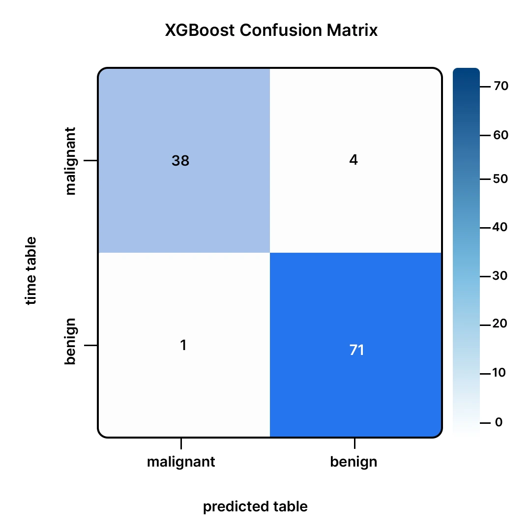
This matrix tells us:

• Out of the 43 malignant tumors (malignant), our model was right in 40 (True Positives).
• It missed 3 malignant tumors, and this is considered to be the most dangerous error because it is an error made on benign tumors (False Negatives).
• Among the 71 benign tumors (benign), our model was right on 69 (True Negatives).
• It also wrongly reported 2 benign tumors as cancer (False Positives).

All in all, this is a great performance. Errors made in the model are minimal.

4. Tuning for Better Performance

We can frequently squeeze more performance by adjusting the hyperparameters of the model. We can attempt to identify a more optimal maxdepth, learning rate, and estimators with the help of the GridSearchCV.

import warnings 
from sklearn.model_selection import GridSearchCV  

warnings.filterwarnings('ignore', category=UserWarning, module='xgboost') 

param_grid = { 
   'max_depth': [3, 6], 
   'learning_rate': [0.1, 0.01], 
   'n_estimators': [50, 100] 
} 

grid_search = GridSearchCV( 
   xgb.XGBClassifier(use_label_encoder=False, eval_metric='logloss', random_state=42), 
   param_grid, scoring='accuracy', cv=3, verbose=1 
) 

grid_search.fit(X_train, y_train); 

print(f"Best parameters: {grid_search.best_params_}") 
best_model = grid_search.best_estimator_ 

# Evaluate the tuned model 
y_pred_best = best_model.predict(X_test) 
best_accuracy = accuracy_score(y_test, y_pred_best) 
print(f"Test Accuracy with best params: {best_accuracy*100:.2f}%") 

Output:

Fitting 3 folds for each of 8 candidates, totalling 24 fits
Best parameters: {'learning_rate': 0.1, 'max_depth': 3, 'n_estimators': 100}
Test Accuracy with best params: 94.74%

Tuning enabled us to find a simpler (max depth of 3 rather than the default depth of 6) model that achieves slightly better performance. This is an excellent result; we achieve more accuracy with a less complex model, and that is less prone to overfitting.

XGBoost includes built-in regularization to reduce overfitting. The two key regularization parameters are:

• lambda (L2 regularization): reg_lambda in the scikit-learn wrapper
• alpha (L1 regularization): reg_alpha in the scikit-learn wrapper

These are official XGBoost parameters used to control model complexity.

Example:

model = xgb.XGBClassifier( 
max_depth=3, 
n_estimators=500, 
learning_rate=0.05, 
reg_lambda=2.0, # stronger L2 regularization 
reg_alpha=0.5, # add L1 regularization 
random_state=42, 
eval_metric="logloss" 
) 

• Increase reg_lambda when the model is overfitting slightly
• Increase reg_alpha if you want more aggressive sparsity in the learned weights and stronger control

Overfitting control

Imagine the XGBoost training as carving. The size of your tools depends on the depth of the trees. Deep trees are sharp tools; they may cut a fine detail, but they may cut errors in the sculpture. The quantity of trees determines the duration of sculpting. More refinements also mean more trees, and as time goes on, you are actually refining noise rather than refining the shape. The rate of learning determines the intensity of each stroke. A smaller learning rate is gentle sculpting: it is slower, safer, and generally cleaner, but requires more strokes (more trees).

The sculpting is the most effective method of preventing overfitting, which is to sculpt gradually and quit at the appropriate moment. Practically, that is by using a lower learning rate, more trees, training by early stopping using a validation set, more sampling (2), and stronger regularisation. Choose more regularisation and sampling to ensure your model is not overconfident in the minute details unlikely to appear in new data.

5. Understanding Feature Importance

One of the best things about tree-based models is that they can produce reports of the most useful features that were used when it came to making a prediction.

# Get and plot feature importances 
importances = best_model.feature_importances_ 
feature_names = data.feature_names 
top_indices = np.argsort(importances)[-10:][::-1]  

plt.figure(figsize=(8, 6)) 
plt.barh(feature_names[top_indices], importances[top_indices], color='skyblue') 
plt.gca().invert_yaxis() 
plt.xlabel("Importance Score") 
plt.title("Top 10 Feature Importances (XGBoost)") 
plt.show() 

Output:

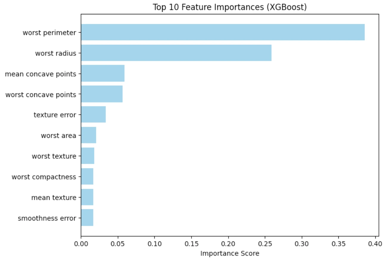
It is clear in the plot that, among the features connected with the geometry of the tumor, the worst concave points and the worst area are the most significant predictors. This is consistent with the medical knowledge and makes us believe that the model is acquiring pertinent patterns.

When NOT to use XGBoost

The XGBoost is a powerful tool, but not necessarily the appropriate one. The following are examples of instances under which you are supposed to take into consideration something other than this:

• When interpretability is a strict requirement: In a regulatory or a medical context, where you need to explain each prediction in a simple manner, then a logistic regression or a little decision tree can fit better.
• When your problem is mostly linear: In case the linear model already does a good job, XGBoost might not make any significant difference without trying to be overly complex.
• When your data is unstructured (images, raw audio, raw text): Deep learning architectures tend to work with raw, unstructured inputs. XGBoost is optimistic in the presence of engineered (structured) features.
• When latency/memory is extremely constrained: An oversized, amplified model may be more heavy than the simpler models.
• When your dataset is extremely small: XGBoost can overfit quickly on tiny datasets unless you tune carefully.

Conclusion

We have learned the reasons why XGBoost is the algorithm of choice for many data scientists. It is a fast and highly performant gradient boosting implementation. We discussed the reasoning behind its sequential and error-correcting process and compared it to other models that are popular.

In our practical example, XGBoost was able to perform quite well even with minimal tuning. The complexity of XGBoost may be very difficult to understand, but it becomes relatively easy to adapt to XGBoost using contemporary libraries. It is possible to make it more than part of your machine learning arsenal, as with practice, it will be prepared to handle your most challenging data problems.

Frequently Asked Questions