An Introduction to Random Forest using the fastai Library (Machine Learning for Programmers – Part 1)

Introduction

Programming is a crucial prerequisite for anyone wanting to learn machine learning. Sure quite a few autoML tools are out there, but most are still at a very nascent stage and well beyond an individual’s budget. The sweet spot for a data scientist lies in combining programming with machine learning algorithms.

Fast.ai is led by the amazing partnership of Jeremy Howard and Rachel Thomas. So when they recently released their machine learning course, I couldn’t wait to get started.

What I personally liked about this course is the top-down approach to teaching. You first learn how to code an algorithm in Python, and then move to the theory aspect. While not a unique approach, it certainly has it’s advantages.

While going these videos, I decided to curate my learning in the form of a series of articles for our awesome community! So in this first post, I have provided a comprehensive summary (including the code) of the first two videos where Jeremy Howard teaches us how to build a random forest model using the fastai library, and how tuning the different hyperparameters can significantly alter our model’s accuracy.

You need to have a bit of experience in Python to follow along with the code. So if you’re a beginner in machine learning and have not used Python and Jupyter Notebooks before, I recommend checking out the below two resources first:

• Introduction to Data Science (covers the basics of Python, Statistics and Predictive Modeling)
• Beginner’s Guide to Jupyter Notebooks

Table of contents

1. Course Structure and Materials
2. Introduction to Machine Learning: Lesson 1
   1. Importing Necessary Libraries
   2. Downloading the Dataset
   3. Introduction to Random Forest
   4. Preprocessing
   5. Model Building
3. Introduction to Machine Learning: Lesson 2
   1. Creating a validation set
   2. Creating a single tree
4. Additional Topics

Course Structure and Materials

The video lectures are available on YouTube and the course has been divided into twelve lectures as per the below structure:

• Lesson 1 – Introduction to Random Forests
• Lesson 2 – Random Forest Deep Dive
• Lesson 3 – Performance, Feature Importance and Model Interpretation
• Lesson 4 – One hot encoding, Partial Dependence, Tree Interpreter
• Lesson 5 – Extrapolation and RF from Scratch
• Lesson 6 – Data Products and Live Coding
• Lesson 7 – RF from Scratch and Gradient Descent
• Lesson 8 – Gradient Descent and Logistic Regression
• Lesson 9 – Regularization, Learning Rates, and NLP
• Lesson 10 – More NLP and Columnar Data
• Lesson 11 – Embeddings
• Lesson 12 – Complete Rossman, Ethical Issues

This course assumes that you have Jupyter Notebook installed on your machine. In case you don’t (and don’t prefer installing it either), you can choose any of the following (these have a nominal fee attached to them):

1. Crestle
2. Paperspace

All the Notebooks associated with each lecture are available on fast.ai’s GitHub repository. You can clone or download the entire repository in one go. You can locate the full installation steps under the to-install section.

Introduction to Machine Learning: Lesson 1

Ready to get started? Then check out the Jupyter Notebook and the below video for the first lesson.

In this lecture, we will learn how to build a random forest model in Python. Since a top-down approach is followed in this course, we will go ahead and code first while simultaneously understanding how the code work. We’ll then look into the inner workings of the random forest algorithm.

Let’s deep dive into what this lecture covers.

Importing necessary libraries

%load ext_autoreload
%autoreload 2

The above two commands will automatically modify the notebook when the source code is updated. Thus, using ext_autoreload will automatically and dynamically make the changes in your notebook.

%matplotlib inline

Using %matplotlib inline, we can visualize the plots inside the notebook.

from fastai.imports import*
from fastai.structured import *
from pandas_summary import DataFrameSummary
from sklearn.ensemble import RandomForestRegressor, RandomForestClassifier
from IPython.display import display
from sklearn import metrics

Using import* will import everything in the fastai library. Other necessary libraries have also been imported for reading the dataframe summary, creating random forest models and metrics for calculating the RMSE (evaluation metric).

Downloading the Dataset

The dataset we’ll be using is the ‘Blue Book for Bulldozers’. The problem statement for this challenge is described below:

The goal is to predict the sale price of a particular piece of heavy equipment at an auction, based on its usage, equipment type, and configuration.  The data is sourced from auction result postings and includes information on usage and equipment configurations. Fast Iron is creating a “blue book for bulldozers”, for customers to value what their heavy equipment fleet is worth at an auction.

The evaluation metric is RMSLE (root mean squared log error). Don’t worry if you haven’t heard of it before, we’ll understand and deal with it during the code walk-through. Assuming you have successfully downloaded the dataset, let’s move on to coding!

PATH = “data/bulldozers/”

This command is used to set the location of our dataset. We currently have the downloaded dataset stored in a folder named bulldozers within the data folder. To check what are the files inside the PATH, you can type:

!ls data/bulldozers/

Or,

!ls {PATH}

Reading the files

The dataset provided is in a .csv format. This is a structured dataset, with columns representing a range of things, such as ID, Date, state, product group, etc. For dealing with structured data, pandas is the most important library. We already imported pandas as pd when we used the import* command earlier. We will now use the read_csv function of pandas to read the data :

df_raw = pd.read_csv(f'{PATH}Train.csv', low_memory=False, parse_dates=["saledate"])

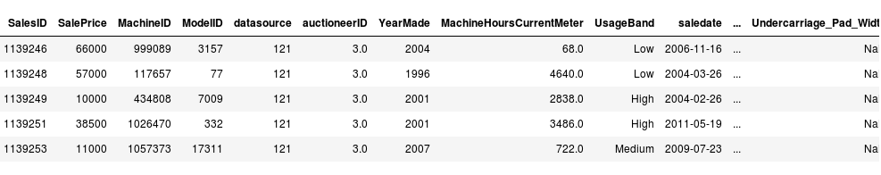
Let us look at the first few rows of the data:

df_raw.head()

Since the dataset is large, this command does not show us the complete column-wise data. Instead, we will see some dots for the data that isn’t being displayed (as shown in the screenshot):

To fix this, we will define the following function, where we set max.rows and max.columns to 1000.

def display_all(df):
    with pd.option_context("display.max_rows", 1000, "display.max_columns", 1000): 
        display(df)

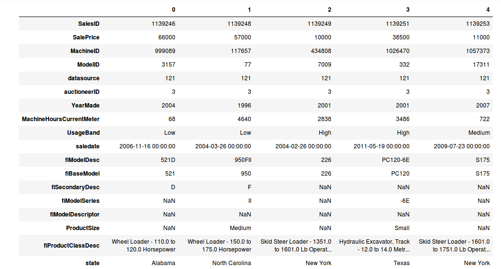
We can now print the head of the dataset using this newly minted function. We have taken the transpose to make it visually appealing (we see column names as the index).

display_all(df_raw.head().transpose())

Remember the evaluation metric is RMSLE – which is basically the RMSE between the log values of the result. So we will transform the target variable by taking it’s log values. This is where the popular library numpy comes to the rescue.

df_raw.SalePrice = np.log(df_raw.SalePrice)

Introduction to Random Forest

The concept of how a Random Forest model works from scratch will be discussed in detail in the later sections of the course, but here is a brief introduction in Jeremy Howard’s words:

• Random forest is a kind of universal machine learning technique
• It can be used for both regression (target is a continuous variable) or classification (target is a categorical variable) problems
• It also works with columns of any kinds, like pixel values, zip codes, revenue, etc.
• In general, random forest does not overfit (it’s very easy to stop it from overfitting)
• You do not need a separate validation set in general. It can tell you how well it generalizes even if you only have one dataset
• It has few (if any) statistical assumptions (it doesn’t assume that data is normally distributed, data is linear, or that you need to specify the interactions)
• Requires very few feature engineering tactics, so it’s a great place to start. For many different types of situations, you do not have to take the log of the data or multiply interactions together

Sounds like a smashing technique, right?

RandomForestRegressor and RandomForestClassifier functions are used in Python for regression and classification problems respectively. Since we’re dealing with a regression challenge, we will stick to the RandomForestRegressor.

m = RandomForestRegressor(n_jobs=-1)
m.fit(df_raw.drop('SalePrice', axis=1), df_raw.SalePrice)

The m.fit function takes two inputs:

• Independent variables
• Dependent (target) variable

The target variable here is df_raw.SalePrice. The independent variables are all the variables except SalePrice. Here, we are using df_raw.drop to drop the SalePrice column (axis = 1 represents column). This would throw up an error like the one below:

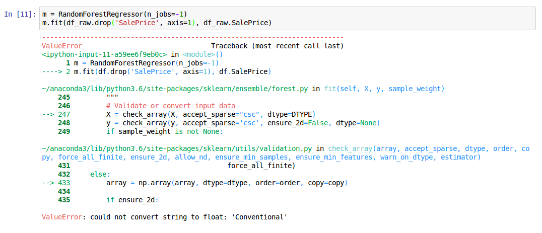
ValueError: could not convert string to float: 'Conventional'

This suggests that the model could not deal with the value ‘Conventional’. Most machine learning models (including random forest) cannot directly use categorical columns. We need to convert these columns into numbers first. So naturally the next step is to convert all the categorical columns into continuous variables.

Data Preprocessing

Let’s take each categorical column individually. First, consider the saledate column which is of datetime format. From the date column, we can extract numerical values such as – year, month, day of month, day of the week, holiday or not, weekend or weekday, was it raining?, etc.

We’ll leverage the add_datepart function from the fastai library to create these features for us. The function creates the following features:

'Year', 'Month', 'Week', 'Day', 'Dayofweek',
'Dayofyear', 'Is_month_end', 'Is_month_start',
'Is_quarter_end', 'Is_quarter_start', 'Is_year_end',
'Is_year_start'

Let’s run the function and check the columns:

add_datepart(df_raw, 'saledate')
df_raw.columns

Index(['SalesID', 'SalePrice', 'MachineID', 'ModelID', 'datasource',
       'auctioneerID', 'YearMade', 'MachineHoursCurrentMeter', 'UsageBand',
       'fiModelDesc', 'fiBaseModel', 'fiSecondaryDesc', 'fiModelSeries',
       'fiModelDescriptor', 'ProductSize', 'fiProductClassDesc', 'state',
       'ProductGroup', 'ProductGroupDesc', 'Drive_System', 'Enclosure',
       'Forks', 'Pad_Type', 'Ride_Control', 'Stick', 'Transmission',
       'Turbocharged', 'Blade_Extension', 'Blade_Width', 'Enclosure_Type',
       'Engine_Horsepower', 'Hydraulics', 'Pushblock', 'Ripper', 'Scarifier',
       'Tip_Control', 'Tire_Size', 'Coupler', 'Coupler_System',
       'Grouser_Tracks', 'Hydraulics_Flow', 'Track_Type',
       'Undercarriage_Pad_Width', 'Stick_Length', 'Thumb', 'Pattern_Changer',
       'Grouser_Type', 'Backhoe_Mounting', 'Blade_Type', 'Travel_Controls',
       'Differential_Type', 'Steering_Controls', 'saleYear', 'saleMonth',
       'saleWeek', 'saleDay', 'saleDayofweek', 'saleDayofyear',
       'saleIs_month_end', 'saleIs_month_start', 'saleIs_quarter_end',
       'saleIs_quarter_start', 'saleIs_year_end', 'saleIs_year_start',
       'saleElapsed'],
      dtype='object')

The next step is to convert the categorical variables into numbers. We can use the train_cats function from fastai for this:

train_cats(df_raw)

While converting categorical to numeric columns, we have to take the following two issues into consideration:

1. Some categorical variables can have an order among them (for example – High>Medium>Low). We can use set_categories to set the order.

   df_raw.UsageBand.cat.set_categories(['High', 'Medium', 'Low'], ordered=True, inplace=True)

2. If a category gets a particular number in the train data, it should have the same value in the test data. For instance, if the train data has 3 for high and test data has 2, then it will have two different meanings. We can use apply_cats for validation and test sets to make sure that the mappings are the same throughout the different sets

Although this won’t make much of a difference in our current case since random forest works on splitting the dataset (we will understand how random forest works in detail in the shortly), it’s still good to know this for other algorithms.

Missing Value Treatment

The next step is to look at the number of missing values in the dataset and understand how to deal with them. This is a pretty widespread challenge in both machine learning competitions and real-life industry problems.

display_all(df_raw.isnull().sum().sort_index()/len(df_raw))

We use .isnull().sum() to get the total number of missing values. This is divided by the length of the dataset to determine the ratio of missing values.

The dataset is now ready to be used for creating a model. Data cleaning is always a tedious and time consuming process. Hence, ensure to save the transformed dataset so that the next time we load the data, we will not have to perform the above tasks again.

We will save it in a feather format, as this let’s us access the data efficiently:

#to save
os.makedirs('tmp', exist_ok=True)
df.to_feather('tmp/bulldozers-raw')

#to read
df_raw = pd.read_feather('tmp/bulldozers-raw')

We have to impute the missing values and store the data as dependent and independent part. This is done by using the fastai function proc_df. The function performs the following tasks:

• For continuous variables, it checks whether a column has missing values or not
• If the column has missing values, it creates another column called columnname_na, which has 1 for missing and 0 for not missing
• Simultaneously, the missing values are replaced with the median of the column
• For categorical variables, pandas replaces missing values with -1. So proc_df adds 1 to all the values for categorical variables. Thus, we have 0 for missing while all other values are incremented by 1

df, y, nas = proc_df(df_raw, 'SalePrice')

Model Building

We have dealt with the categorical columns and the date values. We have also taken care of the missing values. Now we can finally power up and build the random forest model we have been inching towards.

m = RandomForestRegressor(n_jobs=-1)
m.fit(df, y)
m.score(df,y)

The n_jobs is set to -1 to use all the available cores on the machine. This gives us a score (r^2) of 0.98, which is excellent. The caveat here is that we have trained the model on the training set, and checked the result on the same. There’s a high chance that this model might not perform as well on unseen data (test set, in our case).

The only way to find out is to create a validation set and check the performance of the model on it. So let’s create a validation set that contains 12,000 data points (and the train set will contain the rest).

def split_vals(a,n): 
    return a[:n].copy(), a[n:].copy()

n_valid = 12000  # same as Kaggle's test set size
n_trn = len(df)-n_valid
raw_train, raw_valid = split_vals(df_raw, n_trn)
X_train, X_valid = split_vals(df, n_trn)
y_train, y_valid = split_vals(y, n_trn)

X_train.shape, y_train.shape, X_valid.shape

((389125, 66), (389125,), (12000, 66))

Here, we will train the model on our new set (which is a sample of the original set) and check the performance across both – train and validation sets.

#define a function to check rmse value
def rmse(x,y): 
    return math.sqrt(((x-y)**2).mean())

In order to compare the score against the train and test sets, the below function returns the RMSE value and score for both datasets.

def print_score(m):
    res = [rmse(m.predict(X_train), y_train),
           rmse(m.predict(X_valid), y_valid),
           m.score(X_train, y_train), m.score(X_valid, y_valid)]
    if hasattr(m, 'oob_score_'): res.append(m.oob_score_)
    print(res)

m = RandomForestRegressor(n_jobs=-1)
%time m.fit(X_train, y_train)
print_score(m)

The result of the above code is shown below. The train set has a score of 0.98, while the validation set has a score of 0.88. A bit of a drop-off, but the model still performed well overall.

CPU times: user 1min 3s, sys: 356 ms, total: 1min 3s
Wall time: 8.46 s
[0.09044244804386327, 0.2508166961122146, 0.98290459302099709, 0.88765316048270615]

Introduction to Machine Learning: Lesson 2

Now that you know how to code a random forest model in Python, it’s equally important to understand how it actually works underneath all that code. Random forest is often cited as a black box model, and it’s time to put that misconception to bed.

We observed in the first lesson that the model performs extremely well on the training data (the points it has seen before) but dips when tested on the validation set (the data points model was not trained on). Let us first understand how we created the validation set and why it’s so crucial.

Creating a Validation set

Creating a good validation set that closely resembles the test set is one of the most important tasks in machine learning. The validation score is representative of how our model performs on real-world data, or on the test data.

Keep in mind that if there’s a time component involved, then the most recent rows should be included in the validation set. So, our validation set will be of the same size as the test set (last 12,000 rows from the training data).

def split_vals(a,n):
   return a[:n].copy(), a[n:].copy()

n_valid = 12000  
n_trn = len(df)-n_valid
raw_train, raw_valid = split_vals(df_raw, n_trn)
X_train, X_valid = split_vals(df, n_trn)
y_train, y_valid = split_vals(y, n_trn)

The data points from 0 to (length – 12000) are stored as the train set (x_train, y_train). A model is built using the train set and its performance is measured on both the train and validation sets as before.

m = RandomForestRegressor(n_jobs=-1)
%time m.fit(X_train, y_train)
print_score(m)

CPU times: user 1min 3s, sys: 356 ms, total: 1min 3s 
Wall time: 8.46 s 
[0.09044244804386327, 0.2508166961122146, 0.98290459302099709, 0.88765316048270615]

From the above code, we get the results:

• RMSE on the training set
• RMSE on the validation set
• R-square on the training set
• R-square on validation set

It’s clear that the model is overfitting on the training set. Also, it takes a smidge over 1 minute to train. Can we reduce the training time? Yes, we can! To do this, we will further take a subset of the original dataset:

df_trn, y_trn, nas = proc_df(df, 'SalePrice', subset=30000)
X_train, _ = split_vals(df_trn, 20000)
y_train, _ = split_vals(y_trn, 20000)

A subset of 30,000 samples has been created from which we take 20,000 for training the Random Forest model.

Building a single tree

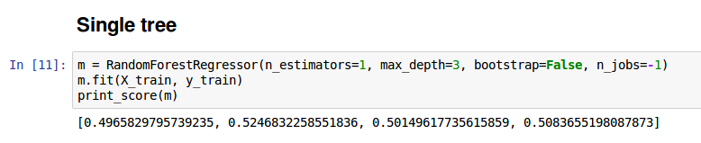
Random Forest is a group of trees which are called estimators. The number of trees in a random forest model is defined by the parameter n_estimator. We will first look at a single tree (set n_estimator = 1) with a maximum depth of 3.

m = RandomForestRegressor(n_estimators=1, max_depth=3, bootstrap=False, n_jobs=-1)
m.fit(X_train, y_train)
print_score(m)

[0.4965829795739235, 0.5246832258551836, 0.50149617735615859, 0.5083655198087873]

Plotting the tree:

draw_tree(m.estimators_[0], df_trn, precision=3)

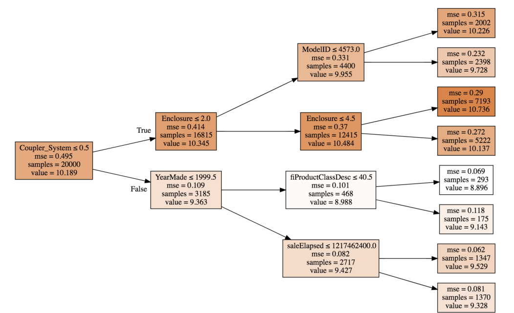
The tree is a set of binary decisions. Looking at the first box, the first split is on coupler-system value: less than/equal to 0.5 or greater than 0.5. After the split, we get 3,185 rows with coupler_system>0.5 and remaining 16,815 with <0.5. Similarly, next split is on enclosure and Year_made.

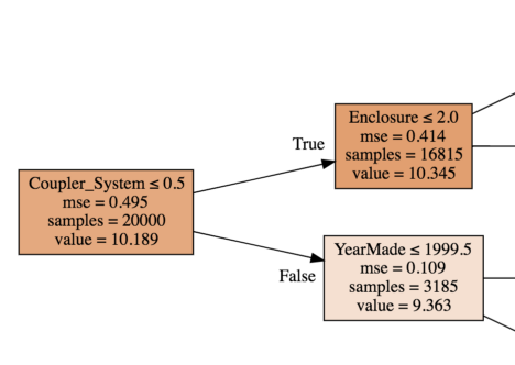
For the first box, a model is created using only the average value (10.189). This means that all the rows have a predicted value of 10.189 and the MSE (Mean Squared Error) for these predictions is 0.459. Instead, if we make a split and separate the rows based on coupler_system <0.5, the MSE is reduced to 0.414 for samples satisfying the condition (true) and 0.109 for the remaining samples.

So how do we decide which variable to split on? The idea is to split the data into two groups which are as different from each other as possible. This can be done by checking each possible split point for each variable, and then figuring out which one gives the lower MSE. To do this, we can take a weighted average of the two MSE values after the split. The splitting stops when it either reaches the pre-specified max_depth value or when each leaf node has only one value.

We have a basic model – a single tree, but this is not a very good model. We need something a bit more complex that builds upon this structure. For creating a forest, we will use a statistical technique called bagging.

Introduction to Bagging

In the bagging technique, we create multiple models, each giving predictions which are not correlated to the other. Then we average the predictions from these models. Random Forest is a bagging technique.

If all the trees created are similar to each other and give similar predictions, then averaging these predictions will not improve the model performance. Instead, we can create multiple trees on a different subset of data, so that even if these trees overfit, they will do so on a different set of points. These samples are taken with replacement.

In simple words, we create multiple poor performing models and average them to create one good model. The individual models must be as predictive as possible, but together should be uncorrelated. We will now increase the number of estimators in our random forest and see the results.

m = RandomForestRegressor(n_jobs=-1)
m.fit(X_train, y_train)
print_score(m)

If we do not give a value to the n_estimator parameter, it is taken as 10 by default. We will get predictions from each of the 10 trees. Further, np.stack will be used to concatenate the predictions one over the other.

preds = np.stack([t.predict(X_valid) for t in m.estimators_])

preds.shape

The dimensions of the predictions is (10, 12000) . This means we have 10 predictions for each row in the validation set.

Now for comparing our model’s results against the validation set, here is the row of predictions, the mean of the predictions and the actual value from validation set.

preds[:,0], np.mean(preds[:,0]), y_valid[0]

The actual value is 9.17 but none of our predictions comes close to this value. On taking the average of all our predictions we get 9.07, which is a better prediction than any of the individual trees.

(array([ 9.21034,  8.9872 , 8.9872 , 8.9872 ,  8.9872 , 9.21034, 8.92266, 9.21034,  9.21034, 8.9872 ]),
9.0700003890739005,
9.1049798563183568)

It’s always a good idea to visualize your model as much as possible. Here is a plot that shows the variation in r^2 value as the number of trees increases.

plt.plot([metrics.r2_score(y_valid, np.mean(preds[:i+1], axis=0)) for i in range(10)]);

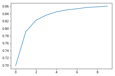
As expected, the r^2 becomes better as the number of trees increases. You can experiment with the n_estimator value and see how the r^2 value changes with each iteration. You’ll notice that after a certain number of trees, the r^2 value plateaus.

Out-of-Bag (OOB) Score

Creating a separate validation set for a small dataset can potentially be a problem since it will result in an even smaller training set. In such cases, we can use the data points (or samples) which the tree was not trained on.

For this, we set the parameter oob_score =True.

m = RandomForestRegressor(n_estimators=40, n_jobs=-1, oob_score=True)
m.fit(X_train, y_train)
print_score(m)

[0.10198464613020647, 0.2714485881623037, 0.9786192457999483, 0.86840992079038759, 0.84831537630038534]

The oob_score is 0.84 which is close to that of the validation set. Let us look at some other interesting techniques by which we can improve our model.

Subsampling

Earlier, we created a subset of 30,000 rows and the train set was randomly chosen from this subset. As an alternative, we can create a different subset each time so that the model is trained on a larger part of the data.

df_trn, y_trn, nas = proc_df(df_raw, 'SalePrice')
X_train, X_valid = split_vals(df_trn, n_trn)
y_train, y_valid = split_vals(y_trn, n_trn)
set_rf_samples(20000)

We use set_rf_sample to specify the sample size. Let us check if the performance of the model has improved or not.

m = RandomForestRegressor(n_estimators=40, n_jobs=-1, oob_score=True)
m.fit(X_train, y_train)
print_score(m)

[0.2317315086850927, 0.26334275954117264, 0.89225792718146846, 0.87615150359885019, 0.88097587673696554]

We get a validation score of 0.876. So far, we have worked on a subset of one sample. We can fit this model on the entire dataset (but it will take a long time to run depending on how good your computational resources are!).

reset_rf_samples()
m = RandomForestRegressor(n_estimators=40, n_jobs=-1, oob_score=True)
m.fit(X_train, y_train)
print_score(m)

[0.07843013746508616, 0.23879806957665775, 0.98490742269867626, 0.89816206196980131, 0.90838819297302553]

Other Hyperparameters to Experiment with and Tune

Min sample leaf

This can be treated as the stopping criteria for the tree. The tree stops growing (or splitting) when the number of samples in the leaf node is less than specified.

m = RandomForestRegressor(n_estimators=40, min_samples_leaf=3,n_jobs=-1, oob_score=True)
m.fit(X_train, y_train)
print_score(m)

[0.11595869956476182, 0.23427349924625201, 0.97209195463880227, 0.90198460308551043, 0.90843297242839738]

Here we have specified the min_sample_leaf as 3. This means that the minimum number of samples in the node should be 3 for each split. We see that the r^2 has improved for the validation set and reduced on the test set, concluding that the model does not overfit on the training data.

Max feature

Another important parameter in random forest is max_features. We have discussed previously that the individual trees must be as uncorrelated as possible. For the same, random forest uses a subset of rows to train each tree. Additionally, we can also use a subset of columns (features) instead of using all the features. This is achieved by tweaking the max_features parameter.

m = RandomForestRegressor(n_estimators=40, min_samples_leaf=3, max_features=0.5, n_jobs=-1, oob_score=True) 
m.fit(X_train, y_train)
print_score(m)

[0.11926975747908228, 0.22869111042050522, 0.97026995966445684, 0.9066000722129437, 0.91144914977164715]

Setting max_features has slightly improved the validation score. Here the max_features is set to 0.5 which means using 50% of the features for each split. Keep in mind that this parameter can also take values like log2 or sqrt.

Additional Topics

Tips and tricks in Jupyter Notebooks

Jeremy Howard mentioned a few tips and tricks for navigating Jupyter Notebooks which newcomers will find quite useful. Below are some of the highlights:

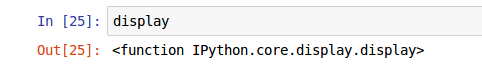
• To find out which library the function is located in, simply type the function name and run the cell (shift-enter):

  display

  

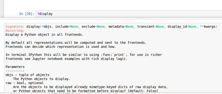
• See the documentation, use a question mark before the function:

  ?display

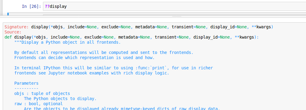
• Check the source code of the function, use a double question mark before the function name:

  ??display

Curse of dimensionality

The curse of dimensionality is the idea that the more dimensions we have, the more points sit on the edge of that space. So if the number of columns is more, it creates more and more empty space. What that means, in theory, is that the distance between points is much less meaningful. This should not be true because the points still are different distances away from each other. Even though they are on the edges, we can still determine how far away they are from each other.

Continuous, categorical, ordinal variables

• Continuous variables are variables with integer or float values. For example – Age, distance, weight, income etc
• Categorical variables are usually strings or values representing names or labels. For example – gender, state, zip code, rank etc
• Ordinal variables are those categorical variables which have an order among them. For example rank (I, II, III ) or remark (poor, good, excellent) have an order.

Overfitting and  Underfitting

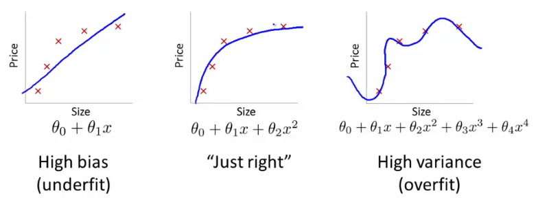
• Underfitting: A model that performs poorly on the train data and also on the test data. The model does not generalize well. (left plot)
• Overfitting: A model that performs extremely well on the train data but does not show a similar high performance on the test data. (right plot)

Root mean squared log error

The evaluation metric of our dataset is RMSLE. The formula for this is

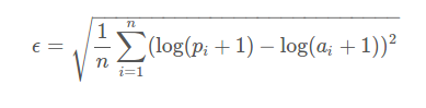
We first take the mean of squared differences of log values. We take a square root of the result obtained. This is equivalent to calculating the root mean squared error (rmse) of log of the values.

R-square

Here is the mathematical formula for R-square:

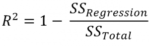
• SS_regression is the sum of squares of (actual value – prediction)
• SS_total is the sum of squares of (actual value – average)

The value of R-square can be anything less than 1. If the r square is negative, it means that your model is worse than predicting mean.

Extremely Randomized Tree

In scikit-learn, we have another algorithm ExtraTreeClassifier which is extremely randomized tree model. Unlike Random forest, instead of trying each split point for every variable, it randomly tries a few split points for a few variables.

End Notes

This article was a pretty comprehensive summary of the first two videos from fast.ai’s machine learning course. During the first lesson we learnt to code a simple random forest model on the bulldozer dataset. Random forest (and most ml algorithms) do not work with categorical variables. We faced a similar problem during the random forest implementation and we saw how can we use the date column and other categorical columns in the dataset for creating a model.

In the second video, the concept of creating a validation set was introduced. We then used this validation set to check the performance of the model and tuned some basic hyper-parameters to improve the model. My favorite part from this video was plotting and visualizing the tree we built. I am sure you would have learnt a lot through these videos. I will shortly post another article covering the next two videos from the course.

Update: Here is part two of the series (Covers Lesson 3, 4 and 5)

An Intuitive Guide to Interpret a Random Forest Model using fastai library (Machine learning for Programmers — Part 2)

Aishwarya Singh

An avid reader and blogger who loves exploring the endless world of data science and artificial intelligence. Fascinated by the limitless applications of ML and AI; eager to learn and discover the depths of data science.