Feature Selection in Machine Learning

Introduction

As a data scientist working with Python, it’s crucial to understand the importance of feature selection when building a machine learning model. In real-life data science problems, it’s almost rare that all the variables in the dataset are useful for building a model. Adding redundant variables reduces the model’s generalization capability and may also reduce the overall accuracy of a classifier. Furthermore, adding more variables to a model increases the overall complexity of the model.

As per the Law of Parsimony of ‘Occam’s Razor’, the best explanation of a problem is that which involves the fewest possible assumptions. Thus, feature selection becomes an indispensable part of building machine learning models.

Learning Objectives:

• Understanding the importance of feature selection.
• Familiarizing with different feature selection techniques.
• Applying feature selection techniques in practice and evaluating performance.

What Is Feature Selection in Machine Learning?

The goal of feature selection techniques in machine learning is to find the best set of features that allows one to build optimized models of studied phenomena.

The techniques for feature selection in machine learning can be broadly classified into the following categories:

Supervised Techniques

These techniques can be used for labeled data and to identify the relevant features for increasing the efficiency of supervised models like classification and regression. For Example- linear regression, decision tree, SVM, etc.

Unsupervised Techniques

These techniques can be used for unlabeled data. For Example- K-Means Clustering, Principal Component Analysis, Hierarchical Clustering, etc.

From a taxonomic point of view, these techniques are classified into filter, wrapper, embedded, and hybrid methods.

Now, let’s discuss some of these popular machine learning feature selection methods in detail.

Types of Feature Selection Methods in ML

Filter Methods

Filter methods pick up the intrinsic properties of the features measured via univariate statistics instead of cross-validation performance. These methods are faster and less computationally expensive than wrapper methods. When dealing with high-dimensional data, it is computationally cheaper to use filter methods.

Let’s, discuss some of these techniques:

Information Gain

Information gain calculates the reduction in entropy from the transformation of a dataset. It can be used for feature selection by evaluating the Information gain of each variable in the context of the target variable.

from sklearn.feature_selection import mutual_info_classif
import matplotlib.pyplot as plt
%matplotlib inline

importances = mutual_info_classif(X, Y)
feat_importances = pd.Series(importances, dataframe.columns[0:len(dataframe.columns)-1])
feat_importances.plot(kind='barh', color = 'teal')
plt.show()

Chi-square Test

The Chi-square test is used for categorical features in a dataset. We calculate Chi-square between each feature and the target and select the desired number of features with the best Chi-square scores. In order to correctly apply the chi-squared to test the relation between various features in the dataset and the target variable, the following conditions have to be met: the variables have to be categorical, sampled independently, and values should have an expected frequency greater than 5.

from sklearn.feature_selection import SelectKBest
from sklearn.feature_selection import chi2

# Convert to categorical data by converting data to integers
X_cat = X.astype(int)

# Three features with highest chi-squared statistics are selected
chi2_features = SelectKBest(chi2, k=3)
X_kbest_features = chi2_features.fit_transform(X_cat, Y)

# Reduced features
print('Original feature number:', X_cat.shape[1])
print('Reduced feature number:', X_kbest_features.shape[1])

Fisher’s Score

Fisher score is one of the most widely used supervised feature selection methods. The algorithm we will use returns the ranks of the variables based on the fisher’s score in descending order. We can then select the variables as per the case.

from skfeature.function.similarity_based import fisher_score
import matplotlib.pyplot as plt
%matplotlib inline

# Calculating scores
ranks = fisher_score.fisher_score(X, Y)

# Plotting the ranks
feat_importances = pd.Series(ranks, dataframe.columns[0:len(dataframe.columns)-1])
feat_importances.plot(kind='barh', color='teal')
plt.show()

Correlation Coefficient

Correlation is a measure of the linear relationship between 2 or more variables. Through correlation, we can predict one variable from the other. The logic behind using correlation for feature selection is that good variables correlate highly with the target. Furthermore, variables should be correlated with the target but uncorrelated among themselves.

If two variables are correlated, we can predict one from the other. Therefore, if two features are correlated, the model only needs one, as the second does not add additional information. We will use the Pearson Correlation here.

import seaborn as sns
import matplotlib.pyplot as plt
%matplotlib inline

# Correlation matrix
cor = dataframe.corr()

# Plotting Heatmap
plt.figure(figsize=(10,6))
sns.heatmap(cor, annot=True)
plt.show()

We need to set an absolute value, say 0.5, as the threshold for selecting the variables. If we find that the predictor variables are correlated, we can drop the variable with a lower correlation coefficient value than the target variable. We can also compute multiple correlation coefficients to check whether more than two variables correlate. This phenomenon is known as multicollinearity.

Variance Threshold

The variance threshold is a simple baseline approach to feature selection. It removes all features whose variance doesn’t meet some threshold. By default, it removes all zero-variance features, i.e., features with the same value in all samples. We assume that features with a higher variance may contain more useful information, but note that we are not taking the relationship between feature variables or feature and target variables into account, which is one of the drawbacks of filter methods.

from sklearn.feature_selection import VarianceThreshold

# Resetting the value of X to make it non-categorical
X = array[:, 0:8]

v_threshold = VarianceThreshold(threshold=0)
v_threshold.fit(X)  # fit finds the features with zero variance
v_threshold.get_support()

The get_support returns a Boolean vector where True means the variable does not have zero variance.

Mean Absolute Difference (MAD)

‘The mean absolute difference (MAD) computes the absolute difference from the mean value. The main difference between the variance and MAD measures is the absence of the square in the latter. The MAD, like the variance, is also a scaled variant.’ [1] This means that the higher the MAD, the higher the discriminatory power.

import numpy as np
import matplotlib.pyplot as plt

# Calculate MAD
mean_abs_diff = np.sum(np.abs(X - np.mean(X, axis=0)), axis=0) / X.shape[0]

# Plot the bar chart
plt.bar(np.arange(X.shape[1]), mean_abs_diff, color='teal')
plt.xlabel("Feature Index")
plt.ylabel("Mean Absolute Deviation")
plt.title("MAD for Each Feature")
plt.show()

Dispersion Ratio

‘Another measure of dispersion applies the arithmetic mean (AM) and the geometric mean (GM). For a given (positive) feature Xi on n patterns, the AM and GM are given by

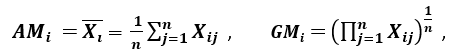respectively; since AMi ≥ GMi, with equality holding if and only if Xi1 = Xi2 = …. = Xin, then the ratio

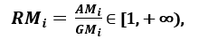
can be used as a dispersion measure. Higher dispersion implies a higher value of Ri, thus a more relevant feature. Conversely, when all the feature samples have (roughly) the same value, Ri is close to 1, indicating a low relevance feature.’ [1]

import numpy as np
import matplotlib.pyplot as plt

# Given data (replace with your actual data)
X = np.array([[1, 2, 3],
              [4, 5, 6],
              [7, 8, 9]])

# Calculate arithmetic mean
am = np.mean(X, axis=0)

# Calculate geometric mean
gm = np.power(np.prod(X, axis=0), 1 / X.shape[0])

# Calculate ratio of arithmetic mean and geometric mean
disp_ratio = am / gm

# Plot the bar chart
plt.bar(np.arange(X.shape[1]), disp_ratio, color='teal')
plt.xlabel("Index")
plt.ylabel("Arithmetic Mean / Geometric Mean")
plt.title("Ratio of Arithmetic Mean and Geometric Mean")
plt.show()

Wrapper Methods

Wrappers require some method to search the space of all possible subsets of features, assessing their quality by learning and evaluating a classifier with that feature subset. The feature selection process is based on a specific machine learning algorithm we are trying to fit on a given dataset. It follows a greedy search approach by evaluating all the possible combinations of features against the evaluation criterion. The wrapper methods usually result in better predictive accuracy than filter methods.

Let’s, discuss some of these techniques:

Forward Feature Selection

This is an iterative method wherein we start with the performing features against the target features. Next, we select another variable that gives the best performance in combination with the first selected variable. This process continues until the preset criterion is achieved.

# Import necessary libraries
from mlxtend.feature_selection import SequentialFeatureSelector

# Create a Sequential Feature Selector object using a logistic regression model
# k_features='best' selects the optimal number of features
# forward=True indicates forward feature selection
# n_jobs=-1 uses all available cores for parallel processing
ffs = SequentialFeatureSelector(lr, k_features='best', forward=True, n_jobs=-1)

# Fit the Sequential Feature Selector to the data
ffs.fit(X, y)

# Get the selected features
features = list(ffs.k_feature_names_)

# Convert feature names to integers (if necessary)
features = list(map(int, features))

# Fit the logistic regression model using only the selected features
lr.fit(X_train[:, features], y_train)

# Make predictions on the training data using the selected features
y_pred = lr.predict(X_train[:, features])

Backward Feature Elimination

This method works exactly opposite to the Forward Feature Selection method. Here, we start with all the features available and build a model. Next, we the variable from the model, which gives the best evaluation measure value. This process is continued until the preset criterion is achieved.

# Import necessary libraries
from sklearn.linear_model import LogisticRegression
from mlxtend.feature_selection import SequentialFeatureSelector

# Create a logistic regression model with class weight balancing
lr = LogisticRegression(class_weight='balanced', solver='lbfgs', random_state=42, n_jobs=-1, max_iter=500)

# Fit the logistic regression model to the data
lr.fit(X, y)

# Create a Sequential Feature Selector object using the logistic regression model
# k_features='best' selects the optimal number of features
# forward=False indicates backward feature selection
# n_jobs=-1 uses all available cores for parallel processing
bfs = SequentialFeatureSelector(lr, k_features='best', forward=False, n_jobs=-1)

# Fit the Sequential Feature Selector to the data
bfs.fit(X, y)

# Get the selected features
features = list(bfs.k_feature_names_)

# Convert feature names to integers (if necessary)
features = list(map(int, features))

# Fit the logistic regression model using only the selected features
lr.fit(X_train[:, features], y_train)

# Make predictions on the training data using the selected features
y_pred = lr.predict(X_train[:, features])

This method, along with the one discussed above, is also known as the Sequential Feature Selection method.

Exhaustive Feature Selection

This is the most robust feature selection method covered so far. This is a brute-force evaluation of each feature subset. This means it tries every possible combination of the variables and returns the best-performing subset.

# Import necessary libraries
from mlxtend.feature_selection import ExhaustiveFeatureSelector
from sklearn.ensemble import RandomForestClassifier

# Create an Exhaustive Feature Selector object using a Random Forest classifier
# min_features=4 sets the minimum number of features to consider
# max_features=8 sets the maximum number of features to consider
# scoring='roc_auc' specifies the scoring metric
# cv=2 specifies the number of cross-validation folds
efs = ExhaustiveFeatureSelector(RandomForestClassifier(), min_features=4, max_features=8, scoring='roc_auc', cv=2)

# Fit the Exhaustive Feature Selector to the data
efs.fit(X, y)

# Print the selected features
selected_features = X_train.columns[list(efs.best_idx_)]
print(selected_features)

# Print the final prediction score
print(efs.best_score_)

Recursive Feature Elimination

‘Given an external estimator that assigns weights to features (e.g., the coefficients of a linear model), the goal of recursive feature elimination (RFE) is to select features by recursively considering smaller and smaller sets of features. First, the estimator is trained on the initial set of features, and each feature’s importance is obtained either through a coef_ attribute or a feature_importances_ attribute.
Then, the least important features are pruned from the current set of features. That procedure is recursively repeated on the pruned set until the desired number of features to select is eventually reached.’

# Import necessary libraries
from sklearn.feature_selection import RFE

# Create a Recursive Feature Elimination object using a logistic regression model
# n_features_to_select=7 specifies the number of features to select
rfe = RFE(lr, n_features_to_select=7)

# Fit the Recursive Feature Elimination object to the data
rfe.fit(X_train, y_train)

# Make predictions on the training data using the selected features
y_pred = rfe.predict(X_train)

Embedded Methods

These methods encompass the benefits of both the wrapper and filter methods by including interactions of features but also maintaining reasonable computational costs. Embedded methods are iterative in the sense that takes care of each iteration of the model training process and carefully extract those features which contribute the most to the training for a particular iteration.

Let’s discuss some of these techniques here:

LASSO Regularization (L1)

Regularization consists of adding a penalty to the different parameters of the machine learning model to reduce the freedom of the model, i.e., to avoid over-fitting. In linear model regularization, the penalty is applied over the coefficients that multiply each predictor. From the different types of regularization, Lasso or L1 has the property that can shrink some of the coefficients to zero. Therefore, that feature can be removed from the model.

# Import necessary libraries
from sklearn.linear_model import LogisticRegression
from sklearn.feature_selection import SelectFromModel

# Create a logistic regression model with L1 regularization
logistic = LogisticRegression(C=1, penalty='l1', solver='liblinear', random_state=7).fit(X, y)

# Create a SelectFromModel object using the logistic regression model
model = SelectFromModel(logistic, prefit=True)

# Transform the feature matrix using the SelectFromModel object
X_new = model.transform(X)

# Get the indices of the selected features
selected_columns = selected_features.columns[selected_features.var() != 0]

# Print the selected features
print(selected_columns)

Random Forest Importance

Random Forests is a kind of Bagging Algorithm that aggregates a specified number of decision trees. The tree-based strategies used by random forests naturally rank by how well they improve the purity of the node, or in other words, a decrease in the impurity (Gini impurity) over all trees. Nodes with the greatest decrease in impurity happen at the start of the trees, while notes with the least decrease in impurity occur at the end of the trees. Thus, by pruning trees below a particular node, we can create a subset of the most important features.

# Import necessary libraries
from sklearn.ensemble import RandomForestClassifier

# Create a Random Forest classifier with your hyperparameters
model = RandomForestClassifier(n_estimators=340)

# Fit the model to the data
model.fit(X, y)

# Get the importance of the resulting features
importances = model.feature_importances_

# Create a data frame for visualization
final_df = pd.DataFrame({'Features': pd.DataFrame(X).columns, 'Importances': importances})
final_df.set_index('Importances')

# Sort in ascending order for better visualization
final_df = final_df.sort_values('Importances')

# Plot the feature importances in bars
final_df.plot.bar(color='teal')

Conclusion

We have discussed a few techniques for feature selection. We have purposely left the feature extraction techniques like Principal Component Analysis, Singular Value Decomposition, Linear Discriminant Analysis, etc. These methods help to reduce the dimensionality of the data or reduce the number of variables while preserving the variance of the data.

Apart from the methods discussed above, there are many other feature selection methods. There are hybrid methods, too, that use both filtering and wrapping techniques. If you wish to explore more about feature selection techniques, great comprehensive reading material, in my opinion, would be ‘Feature Selection for Data and Pattern Recognition’ by Urszula Stańczyk and Lakhmi C. Jain.

Key Takeaways

• Understanding the importance of feature selection and feature engineering in building a machine learning model.
• Familiarizing with different feature selection techniques, including supervised techniques (Information Gain, Chi-square Test, Fisher’s Score, Correlation Coefficient), unsupervised techniques (Variance Threshold, Mean Absolute Difference, Dispersion Ratio), and their classifications (Filter methods, Wrapper methods, Embedded methods, Hybrid methods).
• Evaluating the performance of feature selection techniques in practice through implementation.

Frequently Asked Questions