This article was published as a part of the Data Science Blogathon.
Tried optimizing a large machine learning problem, by some advanced algorithm, and got stuck due to the complexities?! Don’t worry, you have just found the right place. After spending a lot of time behind these and going through some online courses, I’ve found a simpler implementation which I’d like to share with you all.
Introduction
Gradient Descent is one of the most popular and widely used optimization algorithms. Most of you must have implemented it, for finding the values of parameters that will minimize the cost function. In this article, I’ll tell you about some advanced optimization algorithms, through which you can run logistic regression (or even linear regression) much more quickly than gradient descent. Also, this will let the algorithms scale much better, to very large machine learning problems i.e. where we have a large number of features.
For a quick recap, let’s see what gradient descent actually does –
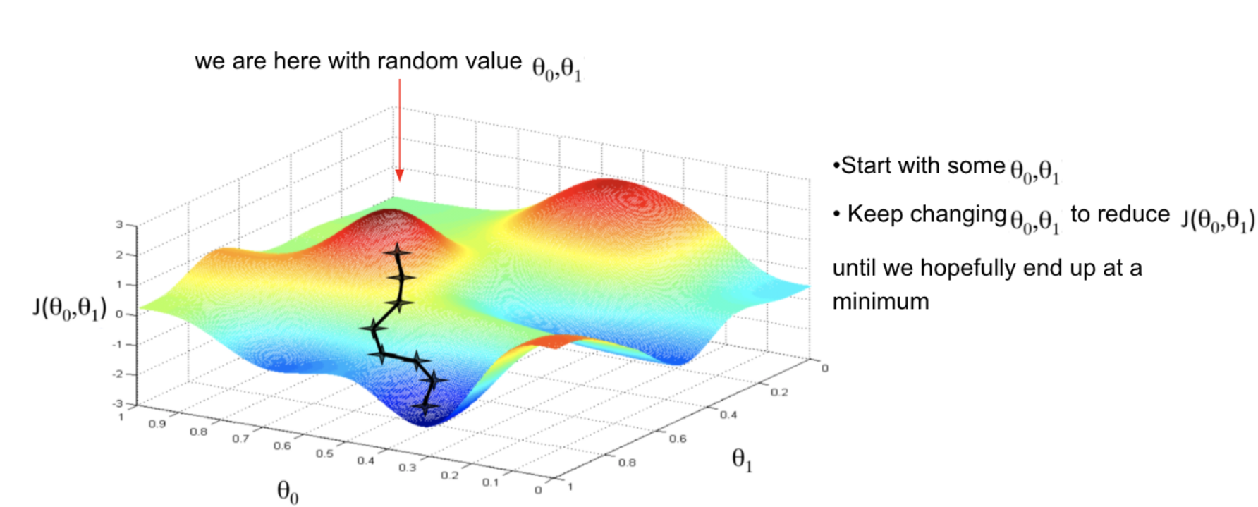
Image source: kdnuggets.com
If we have a cost function, say J, and we want to minimize it. We write a code that takes input parameters, say Θ (theta), and computes J(Θ) and its partial derivatives. So, given the code that does these two things, gradient descent will repeatedly perform an update, to minimize the function for us.
Similarly, there are some advanced algorithms, if we provide a way to compute these two things, they can minimize the cost function with their sophisticated strategies.
Types of Advanced Algorithms
We’ll discuss the three main types of such algorithms which are very useful where a large number of features are involved.
1. Conjugate Gradient:
It is an iterative algorithm, for solving large sparse systems of linear equations. Mainly, it’s used for optimization, neural net training, and image restoration. Theoretically, it is defined as a method that produces an exact solution after a finite number of iterations. However, practically we can’t get the exact solution as it is unstable w.r.t small perturbations. This is a good option for high-dimensional models.
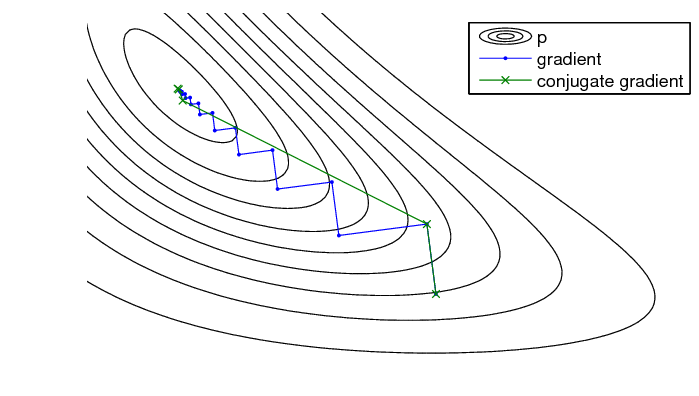
Image source: researchgate.net
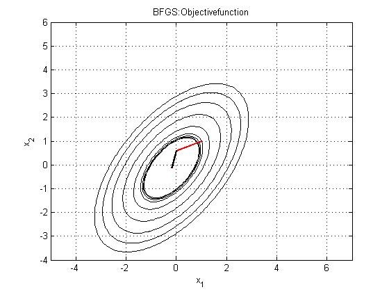
2. BFGS:
It stands for Broyden Fletcher Goldfarb Shanno. It is also an iterative algorithm that is used for solving unconstrained non-linear optimization problems. It basically determines the descent direction, by preconditioning the gradient with curvature information. It is done gradually by improving approximation to the Hessian matrix, of the loss function.
3. L-BFGS:
This is basically a limited memory version of BFGS, mostly suited to problems with many variables (more than 1000). We can get a better solution with a smaller number of iterations. The L-BFGS line search method uses log-linear convergence rates, which reduces the number of line search iterations. This is a good option for low-dimensional models.
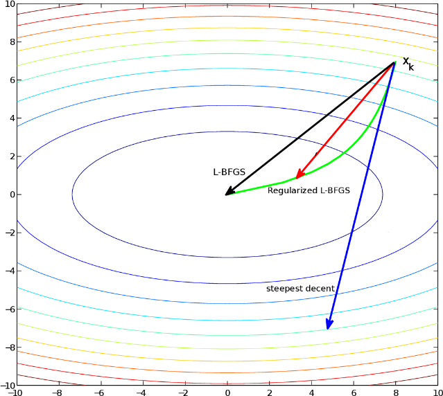
Image source: semanticscholar.org
Advantages and disadvantages over Gradient Descent:
These algorithms have a number of advantages –
1. You don’t have to choose the learning rate manually. They have a clever inter loop called line search algorithm that automatically chooses a good learning rate and even a different learning rate for every iteration.
2. They end up converging much faster than gradient descent.
The only disadvantage is that they are a bit more complex, which makes them less preferred.
Actually, giving a detailed explanation about the working of inter loop and each algorithm separately would take a long time and many more articles!! But, when I searched about those, I found some useful resources through which I figured out that it is possible to use these algorithms successfully without knowing the details of the interloop.
Example and its Implementation
I recommend you to use Octave or MATLAB, as it has a very good library that can implement these algorithms. So, just by using this library, we can get pretty cool results.
Now, I’ll explain how to use these algorithms with an example. Suppose you have been given a problem with two parameters and a cost function as shown below.
- Given problem
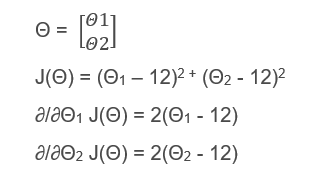
An example showing cost function and its derivatives
In the above figure, we are given Θ (theta) which is a 2×1 vector, a cost function J(Θ) and the last two equations are the partial derivates of the cost function. So, we clearly come to know that the values, Θ1 = 12, Θ2 = 12 will minimize the cost function. Now, we’ll apply one of the advanced optimization algorithms to minimize this cost function and verify the result. I’ll show you an octave function, which can perform this.
- Implementing cost function
function [jVal, gradient] = costFunction(theta)
  jVal = (theta(1)-12)^2 +(theta(2)-12)^2  ;
  gradient = zeros(2,1);
  gradient(1) = 2*(theta(1)-12);
  gradient(2) = 2*(theta(1)-12);
This function basically returns 2 arguments –
1) J-Val: this computes the cost function
2) Gradient: It’s a 2×1 vector. The two elements here correspond to the partial derivative terms (shown above)
Save this code in a file costFunction.m
- Using fminunc()
After implementing the cost function, we can now call the advanced optimization function, fminunc (function minimization unconstrained) in Octave. It is called as shown below –
options = optimset('GradObj','on','MaxIter',100);
initialTheta = zeros(2,1)
[optTheta, functionVal, exitFlag] = fminunc(@costFunction, initialTheta, options)
First, you set options, it is basically like a data structure that stores the options you want. The ‘GradObj’ ‘on’ sets the gradient objective parameter to ON, which means that you will be providing a gradient. I’ve set the maximum iterations to 100. Then, we’ll provide an initial guess for theta, which is a 2×1 vector. The command below it, calls the fminunc function. The ‘@’ symbol there, represents a pointer to the cost function which we defined above. Now, this function, once called, will use one of the advanced optimization algorithms to minimize our cost function.
- Code and output on Octave window
I’ve implemented the above example in Octave and below you can see the command and output.
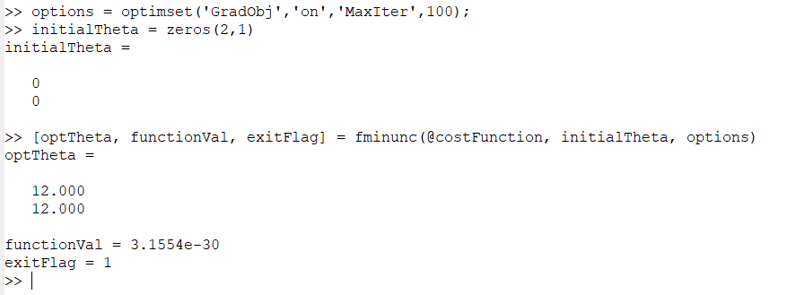
Octave window
As you can see, we got our optimal theta (Θ1 = 12, Θ2 = 12) as we expected. The exit flag basically shows the convergence status, that our algorithm has converged. So, this is the way you can implement these advanced algorithms. Also, I’d like to mention that, this fminunc function will work only if the parameter theta, is a vector and not a real number.
Conclusion
Now you can easily use these advanced optimization algorithms for logistic regression (even linear regression) to work on large problems. As you are using a sophisticated optimization library, it makes it a bit harder to debug, but these run much faster than gradient descent on a large problem. Finally, you have to decide, based on the number of parameters and complexity, which algorithm will be useful for your problem. The first choice is definitely gradient descent, but if you think there are more variables, you can choose stochastic gradient descent, and only for a much larger number of features go for this method.
Thank you for reading!
I hope you enjoyed and learned something new today! Now go on and try
this for a large ML problem. Any comments, suggestions, or ideas are always
welcome. Also, if you find this useful share it with your friends, colleagues and
lastly never stop learning!


