An Effective Approach To Hyper-Parameter Tuning – A Beginners Guide
Introduction To Hyper Parameter Tuning
Hey all,
Let’s say you just entered as a Machine Learning Engineer. Your day-to-day responsibilities involve processing the given analysis to create a deep learning model out of it and embed it into the software in the most miniature time frame possible. Due to numerous projects at hand, you decided to work on problems one by one. However, you soon became overwhelmed by the time to tune the model right and finally became de-motivated.
Well, if you felt the same way, don’t worry, it is a common thing. Even I had the same feeling, so I planned to introduce the technique I used to overcome the issue, and this article is all about it.
By the end of this article, you will have a tool and required knowledge to help you gain an edge in the field. So let’s start.
AGENDA
Here is a quick overview of topics we are going to cover:
1. Understanding Hyper-Parameters (may skip if you know )
2. Our Approach
3 . Implementation:
- 3.1 Basic
- – Loading Libraries
- – Loading dataset + Pre-processing
- – Creating Model(fn) And Quick Evaluation
- 3.2 Tuned
- – Importing Modules
- – Creating H-Param Dictionary + Estimator
- – Fitting to Estimator & Search Optimal
- – Training Optimal
- – Evaluation
4. Tips & Facts
5. References
Having Defined the Agenda, Let’s get started!.
Understanding Hyper-Parameters
A few fundamental questions to ask are: what are hyper-parameters? Why are they essential? and why it’s so time-consuming to work on them. Don’t worry; you will be getting answers to these in this section.
What Are Hyper-Parameters
To understand the analogy of the hyperparameters, let’s compare it with a guitar.
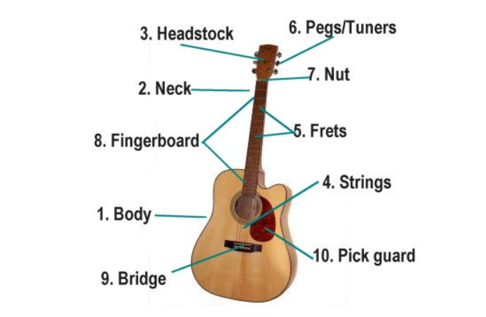
Different Parts of Guitar Explained – credits
In a guitar, you have six strings attached from the bridge(9) to headstock(3) attached to peg/tuners(6). Sounds are produced by plucking these strings, then amplified by the body/ amplifier in electric guitars. Also, the sound quality by the struck place and the tuning of the pegs. So how is this connected to our model? Let me explain if you haven’t understood!
One can think of our hyperparameters as the pegs/tuners, which, when turned right, produced excellent results, in this case, our model.
Why These Are Important
As stated earlier, the H-parameters help our model learn and the representation and data features efficiently, thus contributing to model performance. These are so fragile that even the slightest nudge can result in unexpected performance. Hence one needs to take care of that. Not to forget, for every problem, data, and model, these need to be tuned each time separately.
Why Time Consuming
To understand the time complexity involved, let again head back to our guitar and tune all the possible configurations. Any idea how many combinations?
Well, it’s approx 6- Billion! – for details, refer to this Reddit post. (Doing this is not feasible manually!)
By increasing the no of pegs from 742, you can imagine the time required; that’s why there is so much time involved in the tuning—simple Permutation and Combinations.
Our Approach to understand Hyper-Parameter Tuning
Since we are programmers, we will create a script that will operate instead of manually calculating these. For simplicity, I will be using scikit-learn (Randomized-Search CV), TensorFlow(Keras), and a mnist dataset.
The logic is to create a dictionary of hyperparameters with values as a list. Fitting it to an estimator. Performing a search using optimization algorithm and finally getting results
To perform the evaluation, we will be using mnist-dataset. Also, I divided the implementation part into two: Basic & Tuned.
Implementation in Python
Enough talking, Now let’s see how all the pieces fit into the puzzle. It is good to create a new environment and install the necessary packages mentioned above for the project.
Basics
This section will primarily cover the 3.1 part of the article. The aim is to create a baseline model, which will be later optimized in part 3.2(Tuned).
Loading Libraries
Let’s load some of the necessary libraries and modules(mentioned in the approach part!).
from tensorflow.keras.models import Sequential
from tensorflow.keras.layers import Flatten, Dropout, Dense
from tensorflow.keras.optimizers import Adam
Clarification: Sequential is model type, Flatten, Dropout, and Dense are layers, and Adam is an optimizer.
Loading Data + Pre-Processing
For loading data, we will use the inbuilt Keras mnist dataset.
# importing dataset from keras
from tensorflow.keras.datasets import mnist
# loading dataset
(train_images, train_labels),(test_images, test_labels) = mnist.load_data()
Here mnist.load() will load our data into train and test sets containing data and labels with 60,000 and 10,000 greyscale samples for each.
We now need to change the data type to float32 & rescale our images, i.e., covert each pixel from [0-255] to [0-1].
# conversion +  rescaling
train_data = train_images.astype("float32") / 255
test_data = test_images.astype("float32")/255
To understand what we did, print a single image:
print(train_data[0])
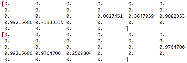
As evident, all values are in the range [0-1], where the change in values represents a change in brightness intensity. Next up, we will create a model fn.
Creating Model fn + Evaluation
Before starting up, it’s essential to understand why we are creating a model fn. Summary: It will return a model for our use each time called, thus allowing for rapid prototyping and architecture change.
So let’s quickly define our fn:
-
# creating model fn
-
def create_model(hidden_layer_one = 784, hidden_layer_two = 256, dropout = 0.2, lr_rate = 0.01):
-
# intializing a sequential model+flattening the input
-
model = Sequential()
-
model.add(Flatten())
-
# creating 1st FFC layer - Dense => Relu => Dropout
-
model.add(Dense(hidden_layer_one, activation = 'relu'))
-
model.add(Dropout(dropout))
-
# creating 2nd FCC layer - Dense => Relu => Dropout
-
model.add(Dense(hidden_layer_two, activation = 'relu'))
-
model.add(Dropout(dropout))
-
# adding a sofmax layer on top
-
model.add(Dense(10, activation = 'softmax'))
-
# compiling model
-
model.compile(optimizer= Adam(learning_rate = lr_rate ),
-
loss = "sparse_categorical_crossentropy",
-
metrics=['accuracy']
-
# returning compiled model
-
return model
For simplicity, code has divided the code into three parts:
Part 1: line 2 – Definition
Our model name is create_model() which accept the following parameters:
- hidden_layer_one – no of nodes in 1st fully connected layers
- hidden_layer_two – no of nodes in 2nd FCC layers
- dropout – value for dropout layer – reduces the over-fitting problem
- lr_rate – learning rate for our optimizer fn. Defines how many steps to take in any direction.
Part 2: line 4-25 – Body
Apart from the parameters to pass, the fn body consists of 2 FCC layers having activation as RELU, followed by dropout layers and a ten-unit(no of digits) dense layer with activation softmax for returning probability.
Finally, the model with loss being ‘sparse_categorical_crossentropy’ll, optimizer as ‘adam,’ and metric to measure is ‘accuracy.‘
For reference, here is a blueprint of our model.
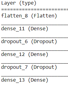
Note: We have passed the num_inputs as parameters(784,256) defined in the function header to allow for a quick change.
By Quickly training our model for 20 epoch, we get an accuracy of 76.50%, which acts as a baseline.
# evaluation - Basic
print("fetching model...")
model = create_model()
print("completed...")
print("training model")
h = model.fit(x = train_data, y= train_labels,
             validation_data = (test_data, test_labels),
             batch_size = 8,
             epochs = 20)
# make predictions on the test set and evaluate it
print("evaluating network...")
accuracy = model.evaluate(test_data, test_labels)[1]
print("accuracy: {:.2f}%".format(accuracy * 100))
In the code above, our model is trained for 20 epochs with a batch size of 8 to ensure faster training.For training same data is used – train(x,y), test(validation).
Finally, the last few lines evaluate the model by giving a single test observation and checking its accuracy, setting the stage for the next part.
Tuned Model
Now let’s perform the optimization to change the accuracy level in this section.
Importing Modules
Before starting, we import some necessary modules.
# import tensorflow and fix the random seed for better reproducibility
import tensorflow as tf
tf.random.set_seed(42)
Imported TensorFlow and set seed for reproducibility.
# import the necessary packages
from tensorflow.keras.wrappers.scikit_learn import KerasClassifier
from sklearn.model_selection import RandomizedSearchCV
Note:
- KerasClassifier: Create multiple models out of model passed
- RandomSearchCV: Searches the optimal value by performing a random search. Accepts a dictionary of parameters
Creating Dictionary + Estimator
The step is like creating a dictionary in python; however, the keys will be similar as passed to out create_model() fn. very important
# define a grid of the hyperparameter search space
HL1 = [256, 512, 784] # num_units 1
HL2 = [128, 256, 512] # num_units 2
LR = [1e-2, 1e-3, 1e-4] # learning rate
DROP = [0.3, 0.4, 0.5] # dropout rate
BATCH_SZ = [4, 8, 16, 32] # batch size
EPOCHS = [10, 20, 30, 40] # epochs
# create a dictionary from the hyperparameter grid
grid = dict(
    hidden_layer_one = HL1,
    hidden_layer_two = HL2,
    dropout = DROP,
    batch_size = BATCH_SZ,
    epochs = EPOCHS)
Next, we need to create an estimator by assigning our create_model() fn to the KerasClassifier.
model = KerasClassifier(build_fn=create_model, verbose=0)
Fitting to Estimator & Search Optimal
Cool, now the only step left is to initialize our search and find the optimal value, performed in the below code.
# 1. start the hyperparameter search process
searcher = RandomizedSearchCV(estimator=model, n_jobs=-1, cv=3,
                             param_distributions=grid, scoring="accuracy")
#2. finding optimal values
searchResults = searcher.fit(train_data, train_labels, verbose = 10)
Understanding the parameters in searcher:
- estimator – create n models
- n_jobs – set no of CPU’s to use, -1 for using all (may slow down pc)
- param_distribution – search space
- scoring – metric to look for – accuracy
In the last code, we initialized our search process by relinquishing the train set. Verbose =1 ensures logs.
Now let’s check the best fit and accuracy by calling the best_params attribute of the searcher.
# summarize grid search information
best_score = searchResults.best_score_
best_params = searchResults.best_params_
print("[INFO] best score is {:.2f} using {}".format(best_score,best_params))
>> [INFO] best score is 0.94 using {‘hidden_layer_two’: 128, ‘hidden_layer_one’: 512, ‘epochs’: 40, ‘dropout’: 0.4, ‘batch_size’: 32}
Ultimately to evaluate the model, a pass of the test-set to score method implies since we have a pre-built model with the best parameters(thanks to our KerasClassifier).
# grabbing the best model
best_model = searchResults.best_estimator_
# checking the accuracy
accuracy = best_model.score(test_data,test_labels)
print("accuracy: {:.2f}%".format(accuracy * 100))
A considerable leap!
Note:
The training time may vary from essential, but it’s still efficient considering the amount of progress it allows. Also, the model’s accuracy will have different values due to the random initialization of the model.
Tips & Facts for Hyper-Parameter Tuning
Here are a few extra tips before walking away :
- Hyper-Parameter is still one of the bottleneck topics in Deep-Learning and seriously, taking it helps!
- This process is highly iterative and performs well when having a small parameter space.
- Many 3rd party libraries like KerasTuner, Optuna, and Ray-Tune are available, which are faster on ample search space.
- The method is fundamental and random, so values one may be slightly off from one represented in the article.
With this, we have come to the end of our article, and I hope you enjoyed reading it and will implement the learned. If you like, consider sharing, and for suggestions, put it down in the comment section. Lastly, here is a few references used article.
References
Code Files: Jupyter-Notebook
Contact: Github | Twitter | LinkedIn
RandomSearch : Documentation
Keras Classifier: Documentation
Inspiration: Code Basics
Hey All✋, My name is Purnendu Shukla a.k.a Harsh. I am a passionate individual who likes exploring & learning new technologies, creating real-life projects, and returning to the community as blogs. My Blogs range from various topics, including Data Science, Machine Learning, Deep Learning, Optimization Problems, Excel and Python Guides, MLOps, Cloud Technologies, Crypto Mining, Quantum Computing.


