This article was published as a part of the Data Science Blogathon.
Introduction to MLIB’s K Means
Most of the machine learning task usually revolves around either the supervised learning approach i.e. the one which gives the label (the column to be predicted) or the unsupervised learning that don’t have any label column in the dataset we have to make relevant groups out of it under certain criteria (choosing the best K value and centroid for each data point).
Similarly, in this article we are going to involve the concept of the unsupervised method more specifically K Means to divide the seeds of wheat into clusters i.e. we have the features of all the wheat seed data though we don’t know to which category they belong to hence clustering technique can help us to segregate that.
About the Dataset
Before going forward with any problem statement it is very much essential that we should get the background and source of the dataset so that the authenticity should sustain. This dataset includes three different categories of what they are, Canadian, Kama, and Rosa. For experiment purposes, 70 features were selected from each of the categories.
If we talk about the image resolution because that is one key area that is highly responsible for the accuracy of the experiment then there was high quality of visualization using the soft X-ray technique and those images were captured by X-ray KODAK plates.
If one needs to know more about this dataset then please visit this link.
This dataset is one of the great examples as it can be used as a clustering task as well as for classification i.e. we can either group different wheat seeds or we can classify which type of wheat seed is this?
Features Information:
To maintain the authentic dataset it is being evaluated from 7 different geometric values. They are as follows
- Area: Denoted by A, have the total area of wheat kernels.
- Perimeter: Denoted by P, consisting of the perimeter.
- Compactness: Denoted by C and the following calculation is done to calculate this aspect = 4piA/P^2.
- Length: Length of the kernel.
- Width: Width of the kernel.
- Asymmetry coefficient: The coefficient value of symmetrical kernels
- Length Kernel: Length of the kernel groove.
Now our main goal is to cluster the wheat seeds into 3 groups using K-means clustering.
Start the practical implementation by setting up the Spark Session.
from pyspark.sql import SparkSession
spark = SparkSession.builder.appName('wheat_seed').getOrCreate()
spark
Output:
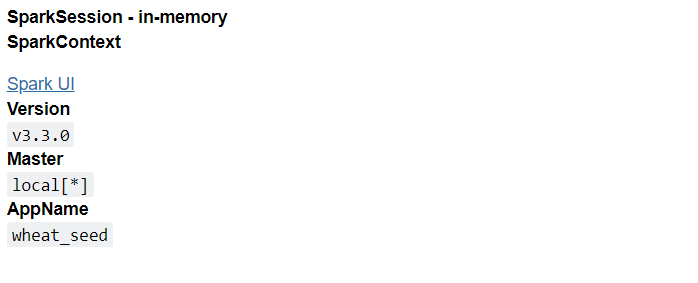
Inference: If anyone is following my PySpark series then by far they are aware of the mandatory steps by which we set up the Spark environment by its PySpark distribution.
Here we gave the name to the session as wheat_seed and created the same using the builder and getOrCreate() method.
from pyspark.ml.clustering import KMeans
Inference: Importing the libraries beforehand is usually recommended so that we don’t fall short of the resources that we need.
Here we are importing specifically the K Means algorithm from the clustering module of PySpark’s MLIB which take in input columns and return the predictions as cluster tag.
Though clustering modules don’t only have the K Means as the options but also LDA, Bisecting K Means, Gaussian Mixture Model, and Power Iteration Clustering.
Reading the Dataset
Let’s read the Wheat seed dataset which is there with us in the CSV format before actually reading it let’s recall a few major points of this dataset.
- It has a total of 7 features or we can say 7 measurements of wheat kernels.
- We already know that in this whole dataset there are 3 types of seeds hence through clustering we just need to give them tags.
dataset = spark.read.csv("seeds_dataset.csv",header=True,inferSchema=True)
dataset.show()
Output:
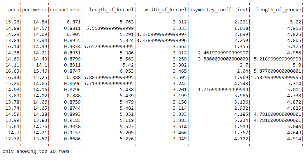
Inference: As usual we used the read.csv function of the PySpark to read the data which was in the CSV format and kept the header parameter as True so that the first column of the dataset should be treated as the column heading. Similarly, inferSchema is also set to True because we want to see the original type of each column.
Note: If we closely look at the above output then we can find out that this dataset requires the “standard scaling” of columns that will be done in the later section of this article.
dataset.head()
Output:
Row(area=15.26, perimeter=14.84, compactness=0.871, length_of_kernel=5.763, width_of_kernel=3.312, asymmetry_coefficient=2.221, length_of_groove=5.22)
Inference: If one wants to see the column name with their corresponding values i.e. tuple of one or more records then the best way is to go with the head() function which will return the Row object which has the records and its values as well.
dataset.describe().show()
Output:
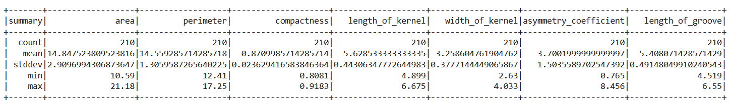
Inference: The describe() method is the go-to function of PySpark when we want to see the statistical information of the dataset. In the above output as well we can see that the total number of instances is 210 and it’s the same for each column which means there are no null values.
Formatting the Data for MLIB
In MLIB we can’t feed all the features to the model in this case we have to first combine all the columns in the vectorized format so that model in the backend can traverse through each numerical value. This clubbing features task is done by VectorAssembler.
from pyspark.ml.linalg import Vectors
from pyspark.ml.feature import VectorAssembler

dataset.columns
Output:
['area',
 'perimeter',
 'compactness',
 'length_of_kernel',
 'width_of_kernel',
 'asymmetry_coefficient',
 'length_of_groove']
Inference: As we need to format our data using Vectors and VectorAssembler so we are importing them from PySpark’s feature module. Also later look at all the available columns which will help us in the following code.
vec_assembler = VectorAssembler(inputCols = dataset.columns, outputCol='features')
final_data = vec_assembler.transform(dataset)
final_data.show()
Output:
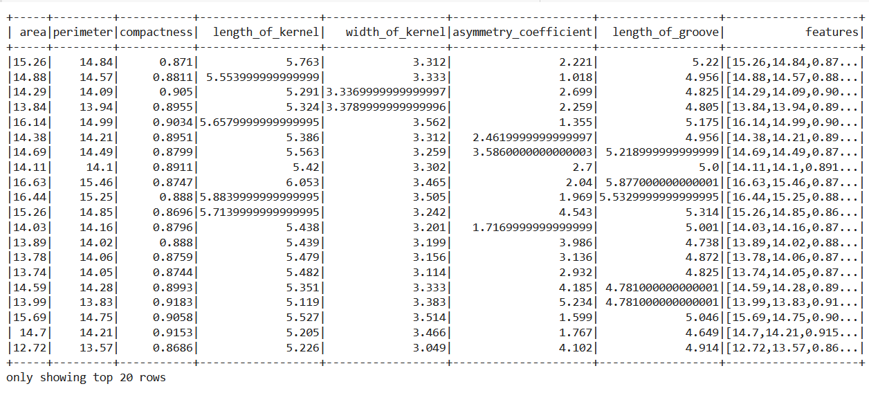
Code breakdown:
- Creating a VectorAssembler object and passing all the columns present in the dataset in the input columns parameter and naming it as the features column.
- Transforming the changes so that they will reflect in the real dataset.
- Then at the last, if we will look at the dataset, the last column is the collection of all the features in the vector.
Scaling the Data
Scaling the data is a completely optional step in the data preprocessing stage but sometimes equally necessary as well depending on the nature of the dataset also scaling down the dataset at the same scale helps to increase the accuracy and deal with the curse of dimensionality.
from pyspark.ml.feature import StandardScaler

scaler = StandardScaler(inputCol="features", outputCol="scaledFeatures", withStd=True, withMean=False)

scalerModel = scaler.fit(final_data)

final_data = scalerModel.transform(final_data)
Code breakdown:
- Importing the StandardScaler object from the ml. feature library of the PySpark.
- Then passing the features as the input column value and scaled features as output column features. The main thing to note here is that we are scaling the data in terms of standard deviation (True) but not with a mean (False).
- In the third step, we are gonna compute the summary statistics by using the fit function.
- In the last step scaled model will normalize every feature to have the same unit of standard deviation.
Training and Evaluating the Model
Now we are actually in the model development phase where first we are gonna build the KMeans clustering model and then for the testing phase, we will evaluate the model using relevant metrics which will let us know how our model performed.
kmeans = KMeans(featuresCol='scaledFeatures',k=3)
model = kmeans.fit(final_data)
model = model.transform(final_data)
Inference: First thing to note is that in the training phase we are passing the k value i.e. several clusters as 3 because we already know that there are 3 types of seeds available.
Then it’s necessary to transform the changes i.e. training the model on the whole dataset (as there are no labels).
from pyspark.ml.evaluation import ClusteringEvaluator
evaluator = ClusteringEvaluator()

silhouette_3_groups = evaluator.evaluate(model)
print("Silhouette evaluation results for wheat seed segmentation= " + str(silhouette_3_groups))
Output:
Silhouette evaluation results for wheat seed segmentation= 0.630000103338996
Inference: Here comes the model evaluation phase where first and foremost we import the ClusteringEvaluator module so that we could statistically check how well the model performed using the Silhouette evaluation measures. The results are neither too good nor too bad. For that one could tune the model and see if it is resulting in better results.
model.select('prediction').show()
Output:
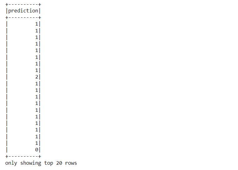
Inference: If one wants to see the tag, like which sets of records belong to what cluster then navigate through the “prediction” column and you can see the results as the above output.
Conclusion on K Means
In the final part of the article where we will go through each step in a brief explanation that helped us to solve the problem of segregating the three types of wheat seeds through K Means clustering.
- Firstly we went through the theory part and learned about the dataset then followed a few compulsory steps like starting the spark session and reading the dataset using PySpark.
- Then after some analysis of the data, we format it to make it ready for the machine learning algorithm ~ K Means clustering.
- When we closely looked at the data we found that it requires standard scaling as well, so after scaling the data we trained it and get through the evaluation part to later reached the conclusion that the model moderately performed.
Here’s the repo link to this article. I hope you liked my article on the Segmentation of wheat crops using MLIB’s K Means. If you have any opinions or questions, then comment below.
Connect with me on LinkedIn for further discussion on MLIB or otherwise.
The media shown in this article is not owned by Analytics Vidhya and is used at the Author’s discretion.


