Comprehensive guide for Data Exploration in R

Introduction

Till now we have already covered a detailed tutorials on data exploration using SAS and Python. What is the one piece missing to complete this series. I am sure you guessed it right. In this article I will give a detailed tutorial on Data Exploration using R. For reader ease, I  will follow a very similar format we used in Python tutorial. This is just because of the sheer resemblance between the two languages.

Here are the operation I’ll cover in this article (Refer to this article for similar operations in SAS):

1. 1. How to load data file(s)?

   2. How to convert a variable to different data type?

   3. How to transpose a table?

   4. How to sort Data?

   5. How to create plots (Histogram, Scatter, Box Plot)?

   6. How to generate frequency tables?

   7. How to do sampling of Data set?

   8. How to remove duplicate values of a variable?

1. How to group variables to calculate count, average, sum?

2. How to recognize and treat missing values and outliers?

3. How to merge / join data set effectively?

 Part 1: How to load data file(s)?

Input data sets can be in various formats (.XLS, .TXT, .CSV, JSON ). In R, it is easy to load data from any source, due to its simple syntax and availability of predefined libraries. Here, I will take examples of reading a CSV file and a tab separated file. read.table is also an alternative, however, read.csv is my preference given the simplicity.

Code:

# Read CSV into R
MyData <- read.csv(file="c:/TheDataIWantToReadIn.csv", header=TRUE, sep=",")
#Read a Tab seperated file
Tabseperated <- read.table("c:/TheDataIWantToReadIn.txt", sep="\t", header=TRUE)

All other Read commands are similar to the one mentioned above.

Part 2: How to convert a variable to different data type?

Type conversions in R work as you would expect. For example, adding a character string to a numeric vector converts all the elements in the vector to character.

Use is.xyz to test for data type xyz. Returns TRUE or FALSE
Use as.xyz to explicitly convert it.

is.numeric(), is.character(), is.vector(), is.matrix(), is.data.frame()
 as.numeric(), as.character(), as.vector(), as.matrix(), as.data.frame()

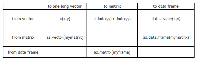
However, conversion of data structure is more critical than the format transformation. Here is grid which will guide you with format conversion :

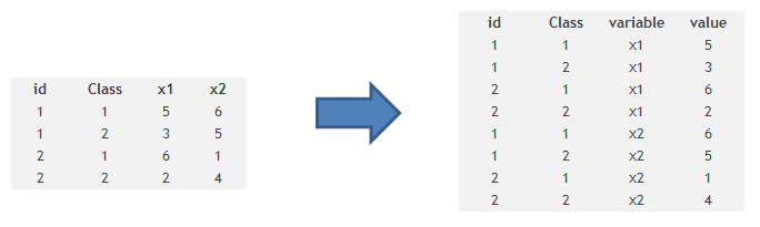
Part 3: How to transpose a Data set?

It is also some times required to transpose a dataset from a wide structure to a narrow structure. Here is the code you use to do the same :

Code

# example of melt function
 library(reshape)
 mdata <- melt(mydata, id=c("id","time"))

Part 4: How to sort DataFrame?

Sorting of data can be done using order(variable name) as an index . It can be based on multiple variables and ascending or descending both order.

Code

# sort by var1
newdata <- old[order(var1),]
# sort by var1 and var2 (descending)
newdata2 <- old[order(var1, -var2),]

Part 5: How to create plots (Histogram)?

Data visualization on R is very easy and creates extremely pretty graphs. Here I will create a distribution of scores in a class and then plot histograms with many variations.

score <-rnorm(n=1000, m=80, sd=20) 
hist(score)

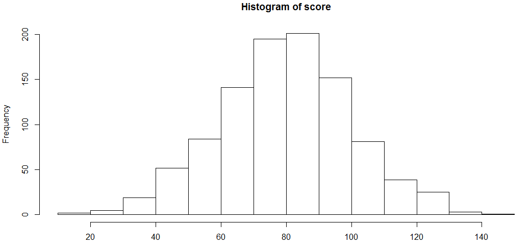
Let’s try to find the assumptions R takes to plot this histogram, and then modify a few of those assumptions.

histinfo<-hist(score)
histinfo

$breaks
 [1] 10 20 30 40 50 60 70 80 90 100 110 120 130 140 150

$counts
 [1] 2 5 19 52 84 141 195 201 152 81 39 25 3 1

$density
 [1] 0.0002 0.0005 0.0019 0.0052 0.0084 0.0141 0.0195 0.0201 0.0152
[10] 0.0081 0.0039 0.0025 0.0003 0.0001

$mids
 [1] 15 25 35 45 55 65 75 85 95 105 115 125 135 145

$xname
[1] "score"

$equidist
[1] TRUE

attr(,"class")
[1] "histogram"

As you can see, the breaks are applied at multiple points. We can restrict the number of break points or vary the density. Over and above this, we can colour the bar plot and overlay a normal distribution curve. Here is how you can do all this :

hist(score, freq=FALSE, xlab="Score", main="Distribution of score", col="lightgreen", xlim=c(0,150), ylim=c(0, 0.02))
curve(dnorm(x, mean=mean(score), sd=sd(score)), add=TRUE, col="darkblue", lwd=2)

Part 6: How to generate frequency tables with R?

Frequency tables are the most basic and effective way to understand distribution across categories.

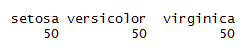
Here is a simple example of calculating one war frequency :

attach(iris)
table(iris$Species)

Here is a code which can find cross tab between two categories :

# 2-Way Cross Tabulation
library(gmodels)
CrossTable(mydata$myrowvar, mydata$mycolvar)

Part 7: How to sample Data set in R?

For sampling a dataset in R, we need to first find a few random indices . Here is how you can find a random sample:

mysample <- mydata[sample(1:nrow(mydata), 100,replace=FALSE),]

This code will simply take out a random sample of 100 observations from the table mydata.

Part 8: How to remove duplicate values of a variable?

Removing duplicates on R is extremely simple. Here is how you do it:

> set.seed(150)
> x <- round(rnorm(20, 10, 5))
> x
 [1] 2 10 6 8 9 11 14 12 11 6 10 0 10 7 7 20 11 17 12 -1
> unique(x)
 [1] 2 10 6 8 9 11 14 12 0 7 20 17 -1

Part 9: How to find class level count average and sum in R?

We generally use Apply functions to do these jobs.

> tapply(iris$Sepal.Length,iris$Species,sum)
 setosa versicolor virginica 
 250.3 296.8 329.4 
> tapply(iris$Sepal.Length,iris$Species,mean)
 setosa versicolor virginica 
 5.006 5.936 6.588

Part 10: How to recognize and Treat missing values and outliers?

Identifying missing values can be done as follows :

> y <- c(4,5,6,NA)
> is.na(y)
[1] FALSE FALSE FALSE TRUE

And here is a quick fix for the same :

y[is.na(y)] <- mean(y,na.rm=TRUE)

y

[1] 4 5 6 5

As you can see, the missing value has been imputed with the mean of other numbers. Similarly, we can impute missing values with any best value available.

Part 11: How to merge / join data sets?

This is yet another operation which we use in our daily life.

To merge two data frames (datasets) horizontally, use the merge function. In most cases, you join two data frames by one or more common key variables (i.e., an inner join).

# merge two data frames by ID
total <- merge(data frameA,data frameB,by="ID")

# merge two data frames by ID and Country
total <- merge(data frameA,data frameB,by=c("ID","Country"))

Appending dataset is another such function which is very frequently used. To join two data frames (datasets) vertically, use the rbind function. The two data frames must have the same variables, but they do not have to be in the same order.

total <- rbind(data frameA, data frameB)

End Notes:

In this comprehensive guide, we looked at the R codes for various steps in data exploration and munging. This tutorial along with the ones available for Python and SAS will give you a comprehensive exposure to the most important languages of the analytics industry.

Did you find the article useful? Do let us know your thoughts about this guide in the comments section below.

If you like what you just read & want to continue your analytics learning, subscribe to our emails, follow us on twitter or like our facebook page.