Introduction
This article navigates the challenges of using Linear Regression for classification problems, emphasizing the unsuitability of Mean Squared Error in Logistic Regression. Explore the mathematics behind Log Loss, a pivotal metric for binary classification models, unraveling its significance and interpretation. With a compelling example involving a clothing company’s predictive modeling, discover the importance of choosing the right model and the complications a linear line introduces in logistic contexts. Gain insights into corrected probabilities and the benefits of logarithms, equipping seasoned data scientists and newcomers for nuanced decision-making in classification tasks.
Learning Objective
- Challenges if we use the Linear Regression model to solve a classification problem.
- Why is MSE not used as a cost function of Logistic Regression?
- This article will cover the mathematics behind the Log Loss formula function with a simple example.
Prerequisites
- Linear Regression
- Logistic Regression
- Gradient Descent
This article was published as a part of the Data Science Blogathon.
Table of contents
What is Log Loss?
Log loss, also known as logarithmic loss or cross-entropy loss, is a common evaluation metric for binary classification models. It measures the performance of a model by quantifying the difference between predicted probabilities and actual values. Log-loss is indicative of how close the prediction probability is to the corresponding actual/true value (0 or 1 in case of binary classification), penalizing inaccurate predictions with higher values. Lower log-loss indicates better model performance.
Log Loss is the most important classification metric based on probabilities. It’s hard to interpret raw log-loss values, but log-loss is still a good metric for comparing models. For any given problem, a lower log loss value means better predictions.
Mathematical interpretation:
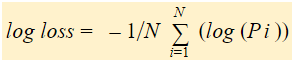
Log Loss is the negative average of the log of corrected predicted probabilities for each instance.
Let us understand it with an example:
What does log loss conceptually mean?
Log loss is a metric evaluating classification model performance by measuring the disparity between predicted and actual probabilities. Rooted in information theory, it penalizes deviations, offering a continuous metric for optimization during model training. Lower log loss values signify better alignment between predicted and actual outcomes, making it a valuable tool for assessing the accuracy of probability estimates in classification problems.
How is a log loss value calculated?
The log loss value is calculated by assessing the likelihood of predicted probabilities matching the actual outcomes in a classification task. For each instance, it computes the negative logarithm of the predicted probability assigned to the correct class. The average of these values across all instances in the dataset yields the final log-loss score. The formula is:
Log Loss=−N1∑i=1N∑j=1Myij⋅log(pij
Here, N is the number of instances, M is the number of classes, yij is a binary indicator (1 if the instance i belongs to class j, 0 otherwise), and pij is the predicted probability that instance i belongs to class j
Let’s Start with an Example
`Winter is here`. Let’s welcome winters with a warm data science problem 😉
Let’s delve into a case study of a clothing company specializing in jackets and cardigans. The company aims to develop a model capable of predicting whether a customer will purchase a jacket (class 1) or a cardigan (class 0) based on their historical behavioral patterns. This predictive model is crucial for tailoring specific offers to meet individual customer needs. As a data scientist, your task is to assist in building this model, considering metrics such as log loss to ensure the accuracy and reliability of predictions.
When we start Machine Learning algorithms, the first algorithm we learn about is `Linear Regression` in which we predict a continuous target variable.
If we use Linear Regression in our classification problem, we will get a best-fit line like this:
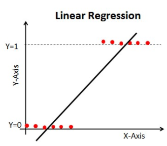
Z = ßX + b
Problem with the Linear Line
When you extend this line, you will have values greater than 1 and less than 0, which do not make much sense in our classification problem. It will make model interpretation a challenge, introducing the risk of misjudging predictions. That is where Logistic Regression, specifically designed for classification tasks and minimizing the log loss, comes in. If we needed to predict sales for an outlet, then this model could be helpful. But here, where our goal is to classify customers, utilizing logistic regression becomes crucial for optimizing performance and minimizing log loss.
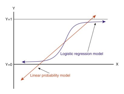
We need a function to transform this straight line in such a way that values will be between 0 and 1:
Ŷ = Q (Z)
Q (Z) =1/1+ e-z (Sigmoid Function)
Ŷ =1/1+ e-z
After transformation, we will get a line that remains between 0 and 1. Another advantage of this function is all the continuous values we will get will be between 0 and 1, making it suitable for applications like log loss, where these values can be utilized as probabilities for making predictions. For example, if the predicted value is on the extreme right, the probability will be close to 1, and if the predicted value is on the extreme left, the probability will be close to 0
Selecting the right model is not enough. You need a function that measures the performance of a Machine Learning model for given data. Cost Function quantifies the error between predicted values and expected values.
`If you can’t measure it, you can’t improve it.`
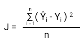
Another thing that will change with this transformation is Cost Function. In Linear Regression, we use `Mean Squared Error` for cost function given by:-
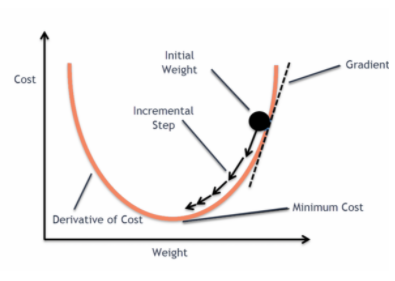
and when this error function is plotted with respect to weight parameters of the Linear Regression Model, it forms a convex curve which makes it eligible to apply Gradient Descent Optimization Algorithm to minimize the error by finding global minima and adjust weights.
Why don’t we use `Mean Squared Error as a cost function in Logistic Regression?
In Logistic Regression Ŷi is a nonlinear function(Ŷ=1/1+ e-z), if we put this in the above MSE equation it will give a non-convex function as shown:
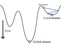
- When we try to optimize values using gradient descent it will create complications to find global minima.
- Another reason is in classification problems, we have target values like 0/1, So (Ŷ-Y)2 will always be in between 0-1 which can make it very difficult to keep track of the errors and it is difficult to store high precision floating numbers.
The cost function used in Logistic Regression is Log Loss.
What are the Corrected Probabilities?
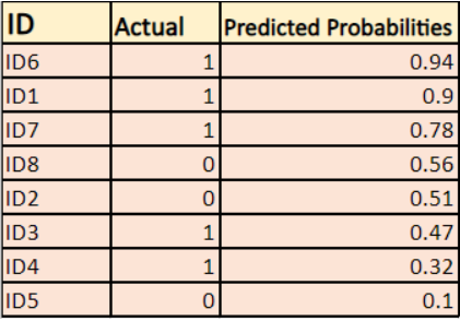
By default, the output of the logistic regression model is the probability of the sample being positive (indicated by 1). For instance, if a logistic regression model is trained to classify a company dataset, the predicted probability column indicates the likelihood of a person buying a jacket. In the given dataset, the log loss for the prediction that a person with ID6 will buy a jacket is 0.94.
In the same way, the probability that a person with ID5 will buy a jacket (i.e. belong to class 1) is 0.1 but the actual class for ID5 is 0, so the probability for the class is (1-0.1)=0.9. 0.9 is the correct probability for ID5.
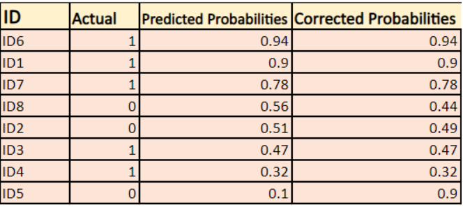
We will find a log of corrected probabilities for each instance.
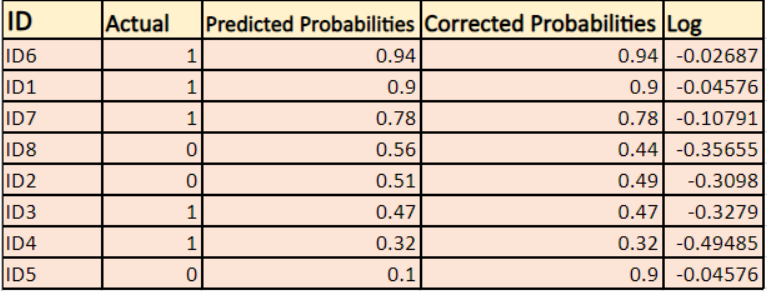
Negative Average
As you can see these log values are negative. To deal with the negative sign, we take the negative average of these values, to maintain a common convention that lower loss scores are better.
In short, there are three steps to find Log Loss:
- To find corrected probabilities.
- Take a log of corrected probabilities.
- Take the negative average of the values we get in the 2nd step.
If we summarize all the above steps, we can use the formula:-
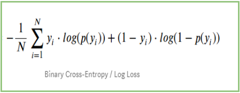
Here Yi represents the actual class and log(p(yi)is the probability of that class.
- p(yi) is the probability of 1.
- 1-p(yi) is the probability of 0.
Now Let’s see how the above formula is working in two cases:
- When the actual class is 1: second term in the formula would be 0 and we will left with first term i.e. yi.log(p(yi)) and (1-1).log(1-p(yi) this will be 0.
- When the actual class is 0: First-term would be 0 and will be left with the second term i.e (1-yi).log(1-p(yi)) and 0.log(p(yi)) will be 0.
wow!! we got back to the original formula for binary cross-entropy/log loss 🙂
The benefits of taking logarithm reveal themselves when you look at the cost function graphs for actual class 1 and 0 :
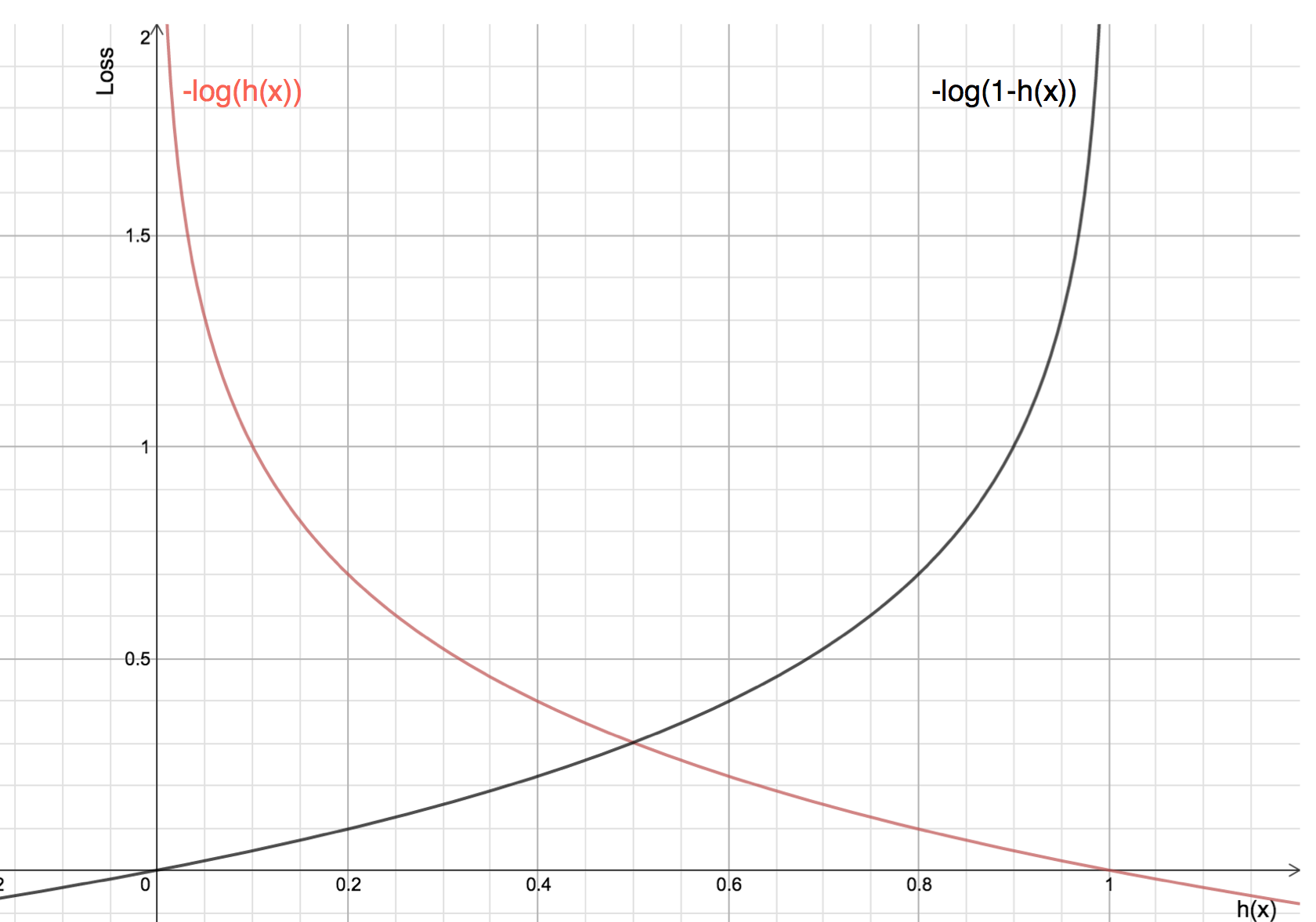
- The Red line represents 1 class. As we can see, when the predicted probability (x-axis) is close to 1, the loss is less and when the predicted probability is close to 0, loss approaches infinity.
- The Black line represents 0 class. As we can see, when the predicted probability (x-axis) is close to 0, the loss is less and when the predicted probability is close to 1, loss approaches infinity.
Frequently Asked Questions
Q1. Why do we use log loss?
A. Log loss is commonly used as an evaluation metric for binary classification tasks for several reasons. Firstly, it provides a continuous and differentiable measure of the model’s performance, making it suitable for optimization algorithms. Secondly, log loss penalizes confident and incorrect predictions more heavily, incentivizing calibrated probability estimates. Finally, log loss can be interpreted as the logarithmic measure of the likelihood of the predicted probabilities aligning with the true labels.
Q2. What is a good log loss?
A. The interpretation of a “good” log loss value depends on the specific context and problem domain. In general, a lower log loss indicates better model performance. However, what constitutes a good log loss can vary depending on the complexity of the problem, the availability of data, and the desired level of accuracy. It is often useful to compare the log loss of different models or benchmarks to assess their relative performance.


Worth reading and great content.
Very well written blog. Short, crisp and equally insightful
That was thoughtful and nicely explained .