This article was published as a part of the Data Science Blogathon.
MLOps is the intersection of Machine Learning, DevOps and Data Engineering.
Introduction:
As the data science and machine learning models are becoming more capable of solving complex business problems, it is evident that many businesses continue to invest in building their capabilities in this field to deliver business value to their users. This trend is also driven by the fact that managing resources such as huge data, infrastructure, compute power, pretrained models, etc have become very inexpensive and on-demand which has enabled teams to go from prototype to production in a very short time.
However, the businesses have also realized that the real challenge isn’t in building machine learning models but on the operational side of things, especially in production. How do we ensure the different pieces of functionalities built by various teams integrate seamlessly? How do make sure that the model in production is not drifting? How do we automatically validate the data from various sources and check for standards? How do we refresh models in production on the fly?
These and many more such questions are not new, and we have seen similar stuff on the typical web development over the years. There have been various methodologies and approaches developed and one such thing is DevOps which has to a large extent addressed these challenges and is the norm currently. So, is there a way to leverage its power in data science?. Let’s explore.
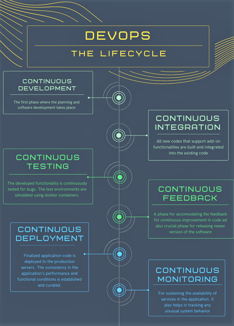
DevOps Lifecycle:
DevOps refers to a software development method and a collaborative way of developing and deploying software. It is a practice that allows a single team to manage the entire application development life cycle, that is, development, testing, deployment, operations. DevOps helps to establish cross-functional teams that share responsibility for maintaining the system that runs the software and prepares the software to run on that system with increased quality feedback and automation issues. At a high level, there are different stages of the DevOps lifecycle.
Here is how all the above components come together to create a seamless development, integration, testing and deployment.
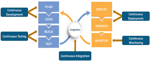
Source: Edureka
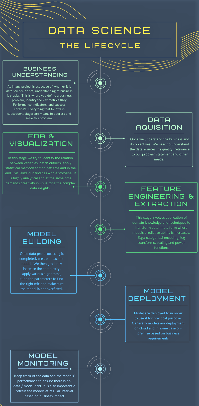
Data Science Lifecycle:
Similar to typical Software Development Lifecycle (SDLC), most data science projects do have a process that outlines the major stages of execution. The lifecycle is not linear meaning each stage may undergo multiple iterations till we reach satisfying results which are acceptable technically and by the business. The various stages of the lifecycle can be summarized below.
Machine Learning Operations (MLOps):
Now, that we have a fair understanding of both DevOps and the Data science lifecycle, is there a way to leverage the powerful features of DevOps like automation, workflows, and test automation in data science projects?
Certainly, yes and that’s what we will explore in the next sections where we will bring these approaches together. In today’s world, this is called Machine Learning Operations (MLOps) and in short, it is the intersection of Machine Learning, DevOps, and Data Engineering. Let’s understand this better with an example.
Any Prerequisites?
To understand MLOps, you will need very basic knowledge of model building in python and a GitHub account. I will be using Visual Studio Code as editor; you can use any editor of your choice as long as you are comfortable with it.
Getting Started:
We will be using Kaggle’s South Africa Heart Disease dataset. Here is the data dictionary for reference. Our objective is to predict chd i.e., coronary heart disease (yes=1 or no=0). A simple binary classification model.
- sbp: systolic blood pressure
- tobacco: cumulative tobacco (kg)
- ldl: low-density lipoprotein cholesterol
- adiposity:
- famhist: family history of heart disease (Present=1, Absent=0)
- typea: type-A behavior
- obesity
- alcohol: current alcohol consumption
- age: age at onset
- chd: coronary heart disease (yes=1 or no=0)
Let’s load the dataset and take a quick look at data and some basic stats. We will also drop ‘famhist‘ variable for now and will experiment with it at a later stage
Python Code:
import pandas as pd

df_heart = pd.read_csv('SAheart.csv', index_col=0)
print(df_heart.head(10))
print(df_heart.describe())
df_heart.drop('famhist', axis=1, inplace=True)

print(df_heart.head())
Split the dataset in train and test:
# Set random seed
seed = 52
# Split into train and test sections
y = df_heart.pop('chd')
X_train, X_test, y_train, y_test = train_test_split(df_heart, y, test_size=0.2, random_state=seed)
Model building: A simple binary classification model
model = LogisticRegression(solver='liblinear', random_state=0).fit(X_train, y_train)
Report training/test score: We will create a text file by name metrics.txt in which the score will be printed
# Report training set score
train_score = model.score(X_train, y_train) * 100

# Report test set score
test_score = model.score(X_test, y_test) * 100

# Write scores to a file
with open("metrics.txt", 'w') as outfile:
outfile.write("Training variance explained: %2.1f%%n" % train_score)
outfile.write("Test variance explained: %2.1f%%n" % test_score)
Model Metrics – Confusion Matrix:
# Confusion Matrix and plot
cm = confusion_matrix(y_test, model.predict(X_test))
fig, ax = plt.subplots(figsize=(8, 8))
ax.imshow(cm)
ax.grid(False)
ax.xaxis.set(ticks=(0, 1), ticklabels=('Predicted 0s', 'Predicted 1s'))
ax.yaxis.set(ticks=(0, 1), ticklabels=('Actual 0s', 'Actual 1s'))
ax.set_ylim(1.5, -0.5)
for i in range(2):
    for j in range(2):
        ax.text(j, i, cm[i, j], ha='center', va='center', color='red')
plt.tight_layout()
plt.savefig("cm.png",dpi=120)
plt.close()
Model Metrics – ROC curve
# Plot the ROC curve
model_ROC = plot_roc_curve(model, X_test, y_test)
plt.tight_layout()
plt.savefig("roc.png",dpi=120)
plt.close()
Classification report to the console: Let’s print this on console, will be handy.
# Print classification report
print(classification_report(y_test, model.predict(X_test)))
Bringing all pieces together: Our final train.py file will be as below
import pandas as pd
from sklearn.linear_model import LogisticRegression
from sklearn.metrics import classification_report, confusion_matrix, roc_auc_score, plot_roc_curve
from sklearn.model_selection import train_test_split
import matplotlib.pyplot as plt
df_heart = pd.read_csv('SAHeart.csv', index_col=0)
df_heart.head(10)
df_heart.describe()
df_heart.drop('famhist', axis=1, inplace=True)
# Set random seed
seed = 52
# Split into train and test sections
y = df_heart.pop('chd')
X_train, X_test, y_train, y_test = train_test_split(df_heart, y, test_size=0.2, random_state=seed)
# Build logistic regression model
model = LogisticRegression(solver='liblinear', random_state=0).fit(X_train, y_train)
# Report training set score
train_score = model.score(X_train, y_train) * 100
# Report test set score
test_score = model.score(X_test, y_test) * 100
# Write scores to a file
with open("metrics.txt", 'w') as outfile:
        outfile.write("Training variance explained: %2.1f%%n" % train_score)
        outfile.write("Test variance explained: %2.1f%%n" % test_score)
# Confusion Matrix and plot
cm = confusion_matrix(y_test, model.predict(X_test))
fig, ax = plt.subplots(figsize=(8, 8))
ax.imshow(cm)
ax.grid(False)
ax.xaxis.set(ticks=(0, 1), ticklabels=('Predicted 0s', 'Predicted 1s'))
ax.yaxis.set(ticks=(0, 1), ticklabels=('Actual 0s', 'Actual 1s'))
ax.set_ylim(1.5, -0.5)
for i in range(2):
    for j in range(2):
        ax.text(j, i, cm[i, j], ha='center', va='center', color='red')
plt.tight_layout()
plt.savefig("cm.png",dpi=120)
plt.close()
# Print classification report
print(classification_report(y_test, model.predict(X_test)))
#roc_auc_score(y_test, model.predict_proba(X_test)[:, 1])
# Plot the ROC curve
model_ROC = plot_roc_curve(model, X_test, y_test)
plt.tight_layout()
plt.savefig("roc.png",dpi=120)
plt.close()
GitHub Workflows and CML: Create a new workflow directory and a new file under it by name cml.yaml. You can name the file anything you want to but ensure the extension is .yaml

Define the process in the yaml as below:
- We want to trigger the process every time there is a code push to the repository.
- We will use the docker image from CML in this case but, we can also use our own docker if required.
- The dependencies that we had defined in requirements.txt file will be installed on the environment.
- Our model file train.py will be executed at the end.
name: model-CHD
on: [push]
jobs:
  run:
    runs-on: [ubuntu-latest]
    container: docker://dvcorg/cml-py3:latest
    steps:
      - uses: actions/checkout@v2
      - name: 'Train my model'
        env:
          repo_token: ${{ secrets.GITHUB_TOKEN }}
        run: |
          # Your ML workflow goes here
          pip install -r requirements.txt
          python train.py
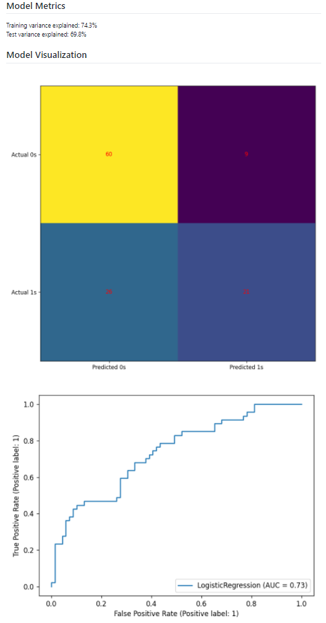
We also had generated some metrics like confusion matrix and ROC curve. It would be great to have them displayed in the markdown format which will help us with our experiments and also to measure/track the model’s performance.
echo "## Model Metrics" >> report.md
cat metrics.txt >> report.md
# Write your CML report
echo "## Model Visualization" >> report.md
cml-publish cm.png --md >> report.md
cml-publish roc.png --md >> report.md
cml-send-comment report.md
Refer to the complete YAML file from the git repository.
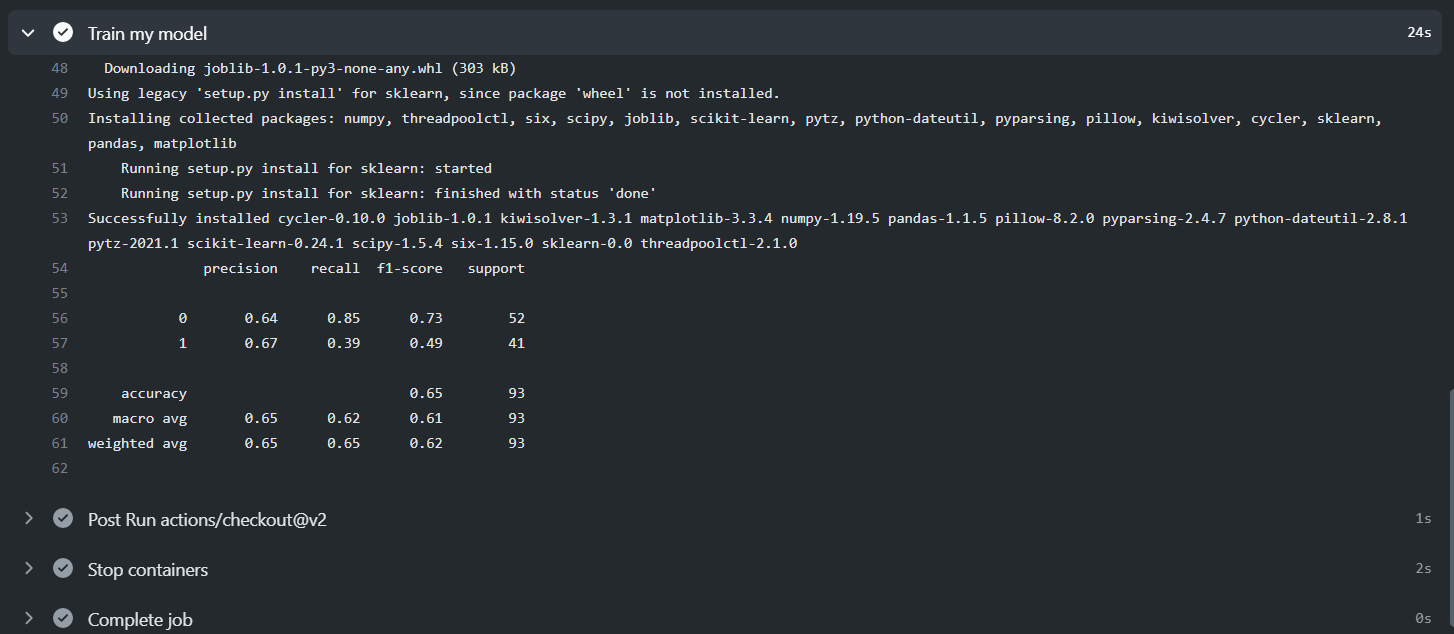
Once you commit the YAML file, the workflow will be triggered as shown below.
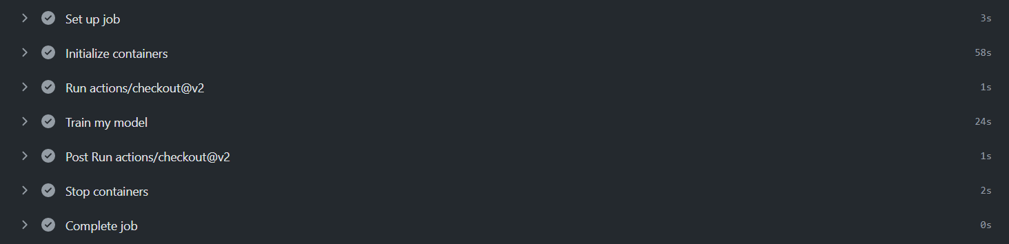
Expand the Train my model tab and there is our classification report we had planned to print on the console.
Navigate your commits on GitHub and you can see the results and both the plots in markdown format.

Great, we have been able to load the data, build a model, create a workflow, and execute the whole process on git push.
Now, let’s experiment: Once we make any changes to the code and push it to GitHub, the entire workflow will be triggered and a new markdown report will be generated specific to our experiment.
- we will change the test size from 0.2 to 0.25
X_train, X_test, y_train, y_test = train_test_split(df_heart, y, test_size=0.25, random_state=seed)
- We had initially dropped a variable by name famhist, lets dummy it and use it in our model
df_heart = pd.get_dummies(df_heart, columns = ['famhist'], drop_first=True)
Ahh!!! As you can see, there is an improvement in the model’s performance with our changes using MLOps.
Conclusion:
The objective of the blog was to showcase how we can leverage the powerful features of DevOps like CI/CD, automation, workflows and apply them to our data science projects & experiments with MLOps. The CML – Continuous Machine Learning is a very handy tool have for tracking the experiment results, collaborate with others, and automating the entire workflow.
Happy learnings !!!!
You can connect with me – Linkedin
You can find the code for reference – Github
References
https://docs.github.com/en/actions
The media shown in this article are not owned by Analytics Vidhya and is used at the Author’s discretion.
I am a Data Science enthusiast with experience in building predictive models, data processing, and data mining algorithms to solve challenging business problems. Involved in open source community and passionate about building data apps.


Excellent blog to illustrate the concept of MLOPs . New to this ML field and still learning git and DevOps. Found it extremely useful. clone the rep and then played around with a few changes and checked the build, metrics generation and plots updated accordingly automatically. Thanks so much for this
This is a very interesting blog post, but I do miss the integration of this project into existing software. It's good to automatically train this model, but is the trained model ever saved and loaded into production? If you want to check this model with new data while it is already in production, let's say by using an API, how will this be done? I am interested into your insights on that.