Linear Regression for Absolute Beginners with Implementation in Python!

This article was published as a part of the Data Science Blogathon.

Warning: This article is for absolute beginners, I assume you just entered into the field of machine learning with some knowledge of high school mathematics and some basic coding but that’s not even mandatory.

Introduction

Linear Regression is the most basic supervised machine learning algorithm. Supervise in the sense that the algorithm can answer your question based on labeled data that you feed to the algorithm. The answer would be like predicting housing prices, classifying dogs vs cats. Here we are going to talk about a regression task using Linear Regression. In the end, we are going to predict housing prices based on the area of the house.

I don’t want to bore you by throwing all the machine learning jargon words, in the beginning, So let me start with the most basic linear equation (y=mx+b) that we all are familiar with since our school time.

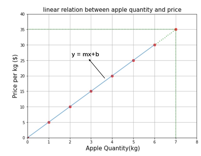
The figure above shows the relationship between the quantity of apple and the cost price. How much do you need to pay for 7kg of apples? I know it’s easy. If 1kg costs 5$ then 7kg cost 7*5=35$ or you will just draw a perpendicular line from point 7 along the y-axis until it touches the linear equation and the corresponding value on the y-axis is the answer as shown by the green dotted line on the graph. But we are going to solve using the formula of a linear equation.

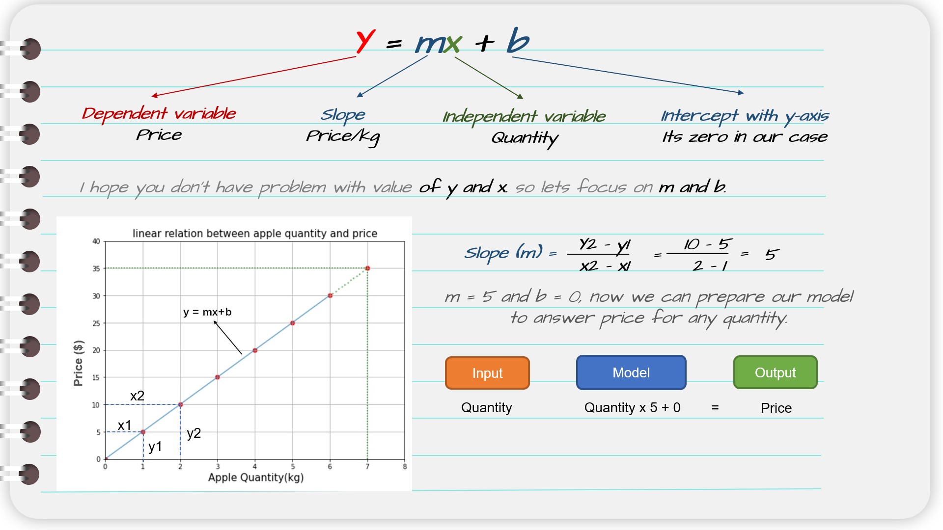
Now, if I have to find the price of 9.5 kg of apple then according to our model mx+b = 5 * 9.5 + 0 = $47.5 is the answer. By now you might have understood that m and b are the main ingredients of the linear equation or in other words m and b are called parameters.

Unfortunately, this is not the machine learning problem neither linear equation is prediction algorithm, But luckily linear regression outputs the result the same way as the linear equation does. The main purpose of the linear regression algorithm is to find the value of m and b that fit the model and after that same m and b are used to predict the result for the given input data.

Predict housing prices

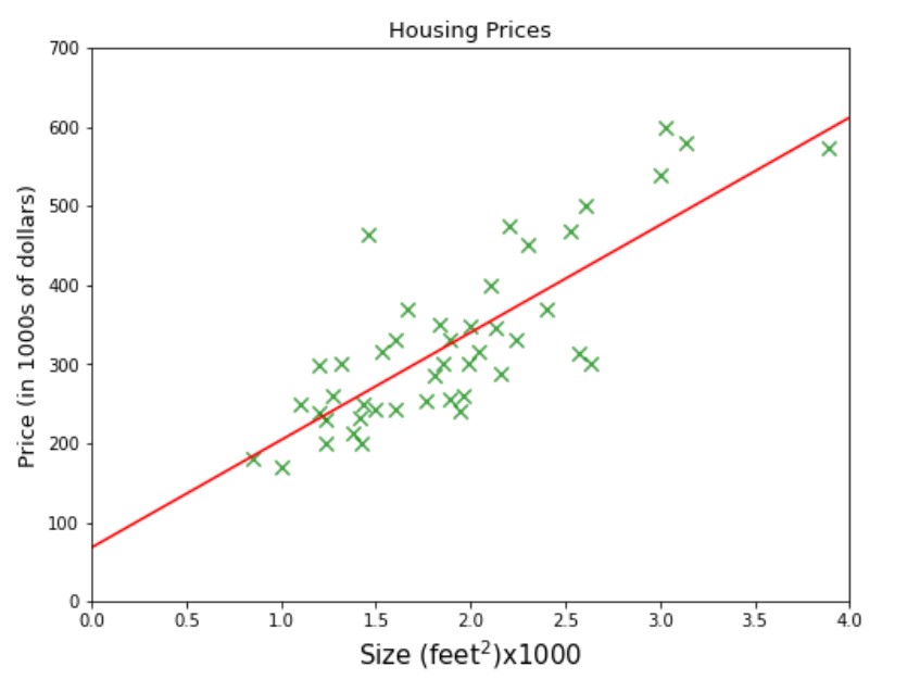
Now we are going to dive a little deeper into solving the regression problem. Look at the data samples or also termed as training examples given in the figure below.

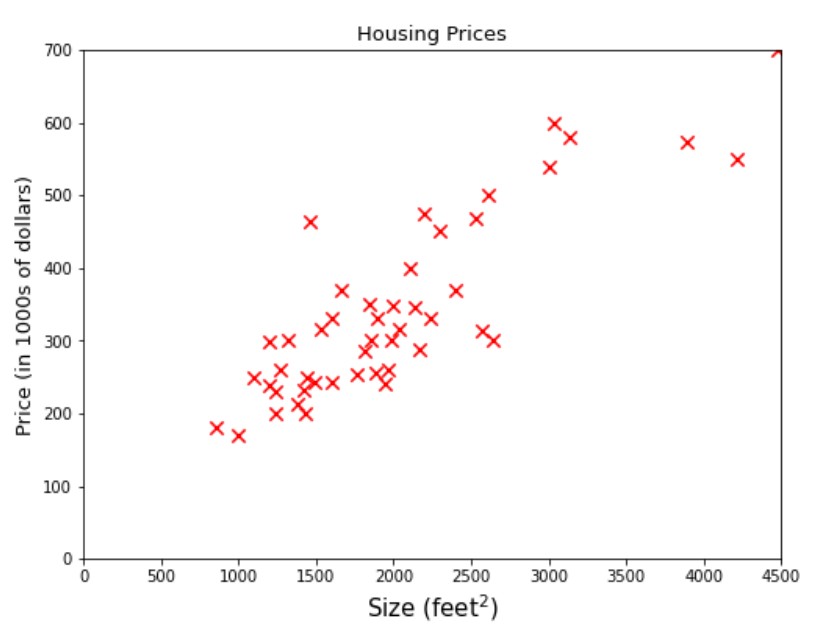
A company name ABC provides you a data on the houses’ size and its price. The company requires providing them a machine learning model that can predict houses’ prices for any given size. Let’s say what would be the best-estimated price for area 3000 feet square? If you are thinking to fit a line somewhere between the dataset and draw a verticle line from 3000 on the x-axis until it touches the line and then the corresponding value on the y-axis i.e 470 would be the answer, then you are on right track, it is represented by the green dotted line in the figure below.

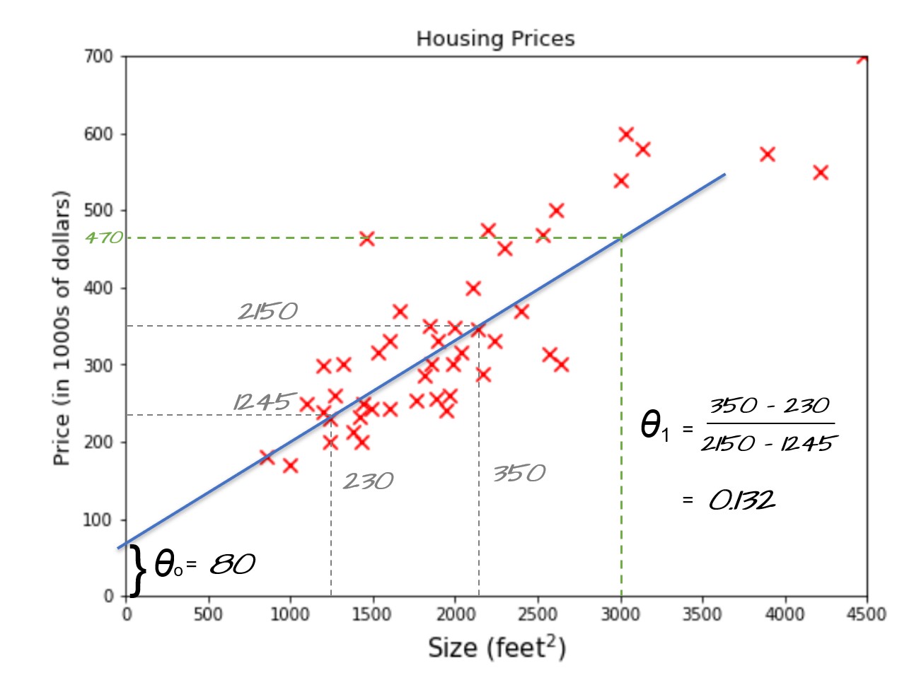
Let’s do it in another way, if we could find the equation of line y = mx+b that we use to fit the data represented by the blue inclined line then we can easily find the model that can predict the housing prices for any given area. In machine learning lingo function y = mx+b is also called a hypothesis function where m and b can be represented by theta0 and theta1 respectively. theta0 is also called a bias term and theta1,theta2,.. are called weights.

See the blue line in the picture above, By taking any two samples that touch or very close to the line we can find the theta1 (slope) = 0.132 and theta zero = 80 as shown in the figure. Now we can use our hypothesis function to predict housing price for size 3000 feet square i.e 80+3000*0.132 = 476. $476,000 could be the best-estimated price for a house of size 3000 feet square and this could be a reasonable way to prepare a machine learning model when you have just 50 samples and with only one feature(size).

But the real-world dataset could be in the order of thousands or even in millions and the number of features could range from (5–100) or even in thousands. At that time our intuition won’t be useful to find thousands of parameters just by looking at a dataset that’s why we need a machine-learning algorithm to carry out such a complex calculation. Grab a cup of coffee, refresh yourself and come back again because from now onwards you are going to understand the way the algorithm works and you will be introduced to a lot of new terminologies. Get ready!!

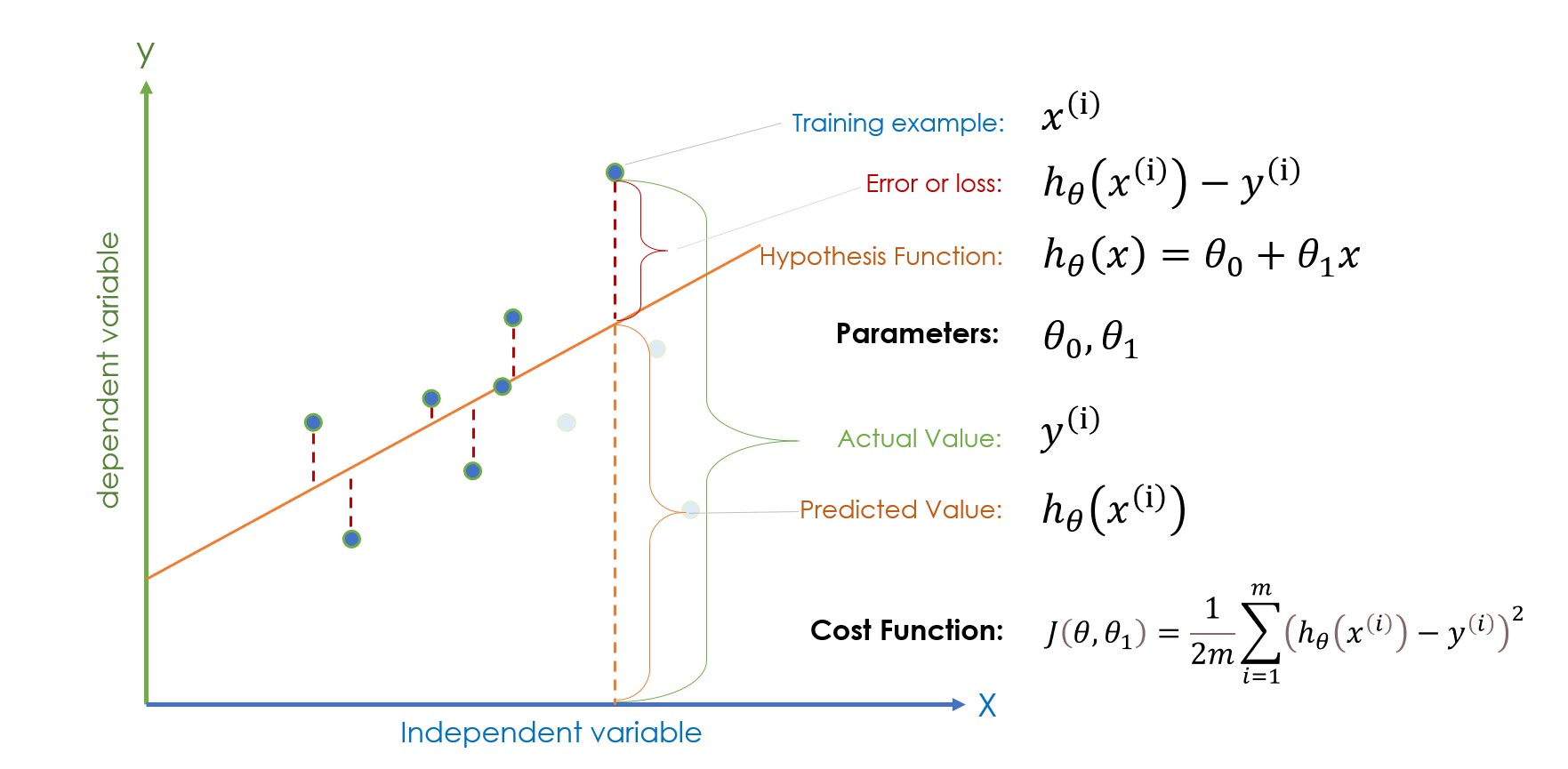
Note: (i) in the equation represents the ith training example, not the power.

If the terminologies given in the above figure seem like aliens to you please take a few minutes to familiarize yourself and try to find a connection with each term. If you know to some extent let’s move ahead. Once the parameter values i.e bias term and theta1 are randomly initialized, the hypothesis function is ready for prediction, and then the error (|predicted value – actual value|) is calculated to check whether the randomly initialized parameter is giving the right prediction or not.

If the error is too high, then the algorithm updates the parameters with a new value, if the error is high again it will update the parameters with the new value again. The algorithm continues this process until the error is minimized. To minimize the error we have a special function called Gradient Descent but before that, we are going to understand what Cost Function is and how it works?

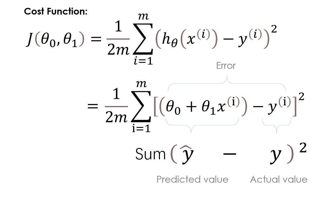
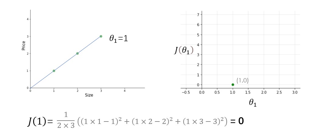
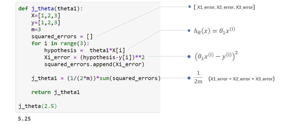
Here in the cost function, we are trying to find the square of the differences between the predicted value and actual value of each training example and then summing up all the differences together or in other words, we are finding the square of error of each training example and then summing up all the errors together. The output we get is simply the mean squared error of a particular set of parameters. Ok, no more words let’s do the calculation. For the simplicity of calculation, we are going to use just one parameter theta1 and a very simple dataset.

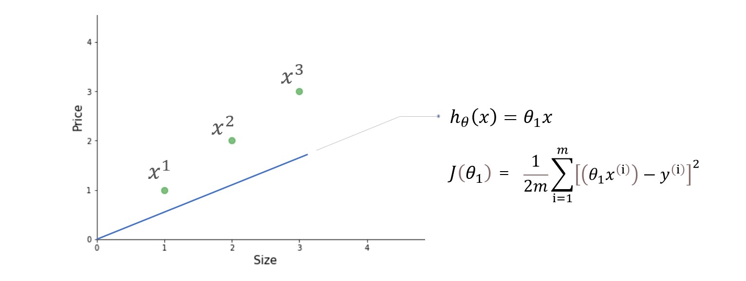
We have three training examples (X1=1, y1=1), (X2=2, y2=2), and (X3=3, y3=3). figure on the left is of hypothesis function and on the right is cost function plotted for different values of the parameter.

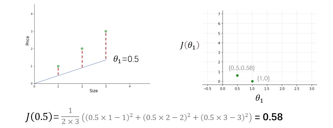
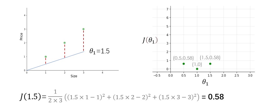
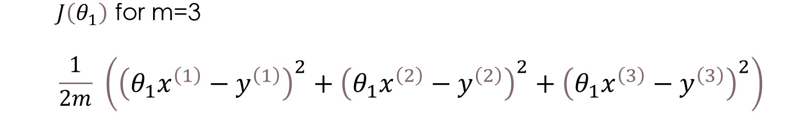
Try other values of theta1 yourself and calculate the cost for each theta1 value. Once you plot these all dots, the cost function will look like a bowl-shaped curve as shown in the figure below.

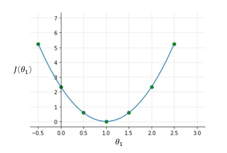
From the figure and calculation, it is clear that the cost function is minimum at theta1=1 or at the bottom of the bowl-shaped curve. The purpose of all this hard work is not to calculate the minimum value of cost function, we have a better way to do this, instead try to understand the relationship between parameters, hypothesis function, and cost function. Please make sure you understand all these concepts before moving ahead.

Coding Cost Function:

 

Gradient Descent:

Why do we need a Gradient Descent?

• In short to minimize the cost function, But How? Let’s see

The cost function only works when it knows the parameters’ values, In the above sample example we manually choose the parameters’ value each time but during the algorithmic calculation once the parameters’ values are randomly initialized it’s the gradient descent who have to decide what params value to choose in the next iteration in order to minimize the error, it’s the gradient descent who decide by how much to increase or decrease the params values.

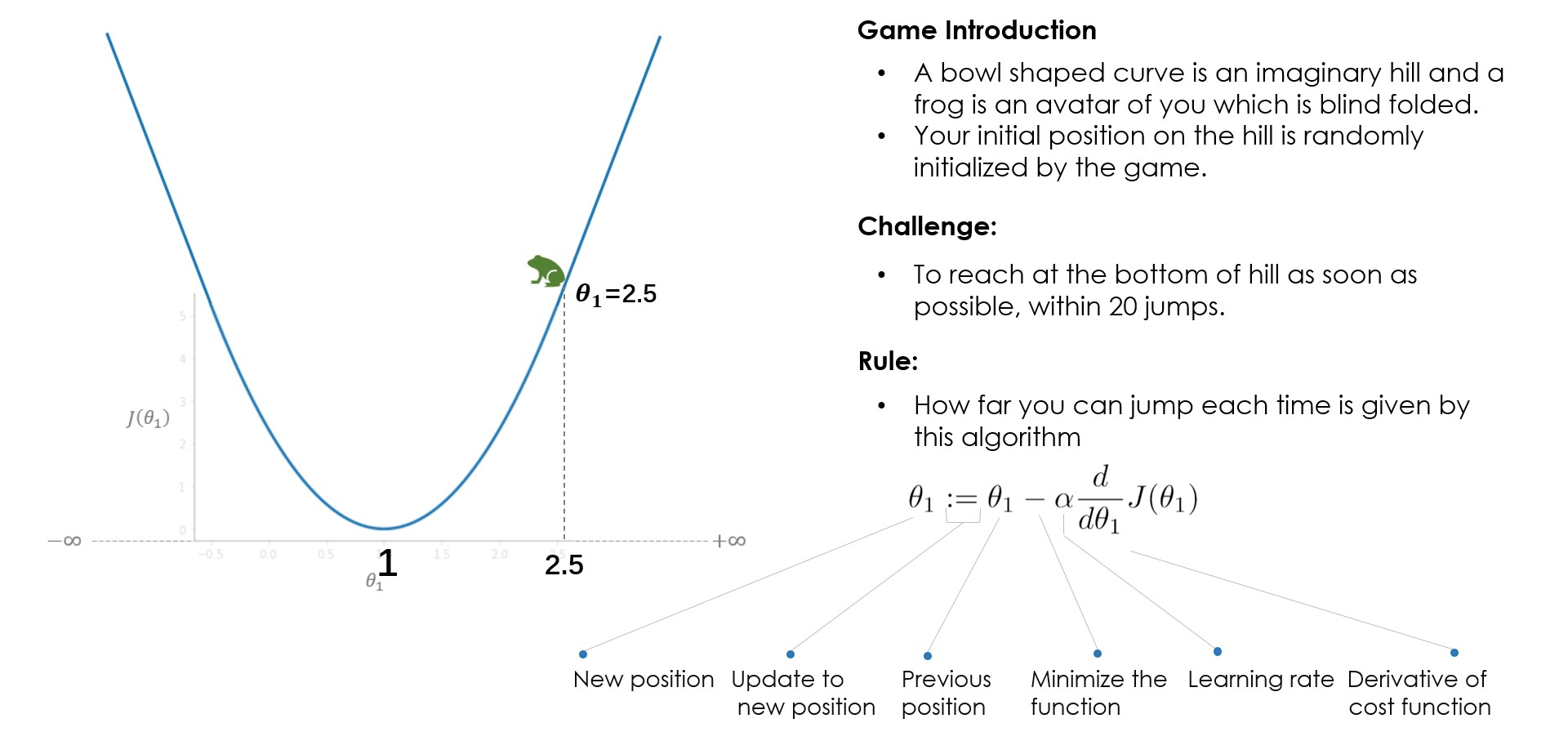
Analogy: How Gradient Descent works?

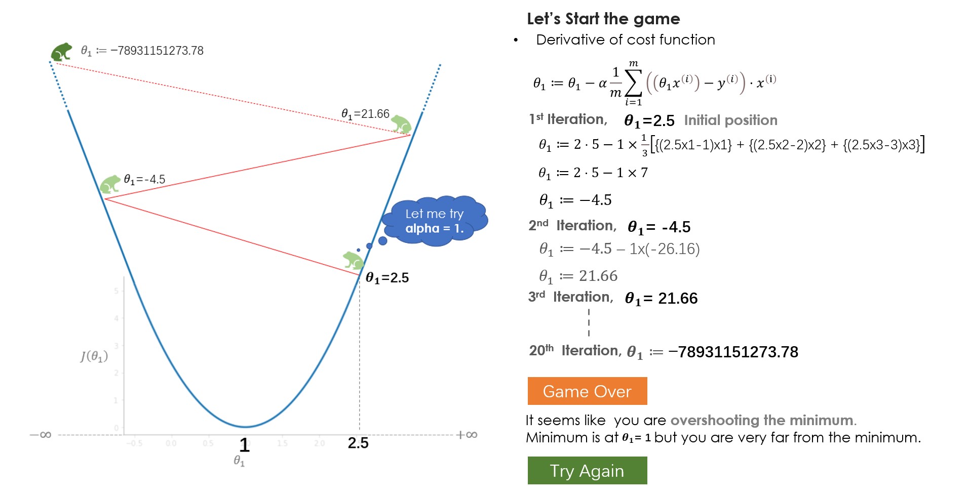
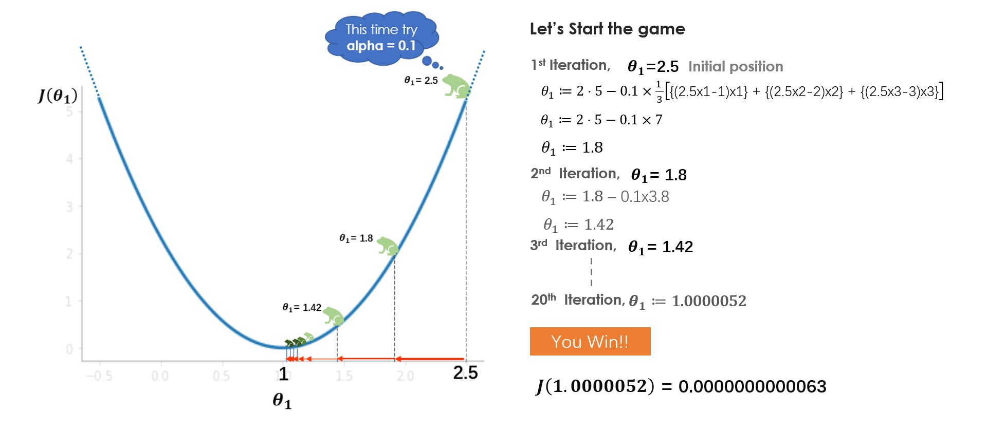
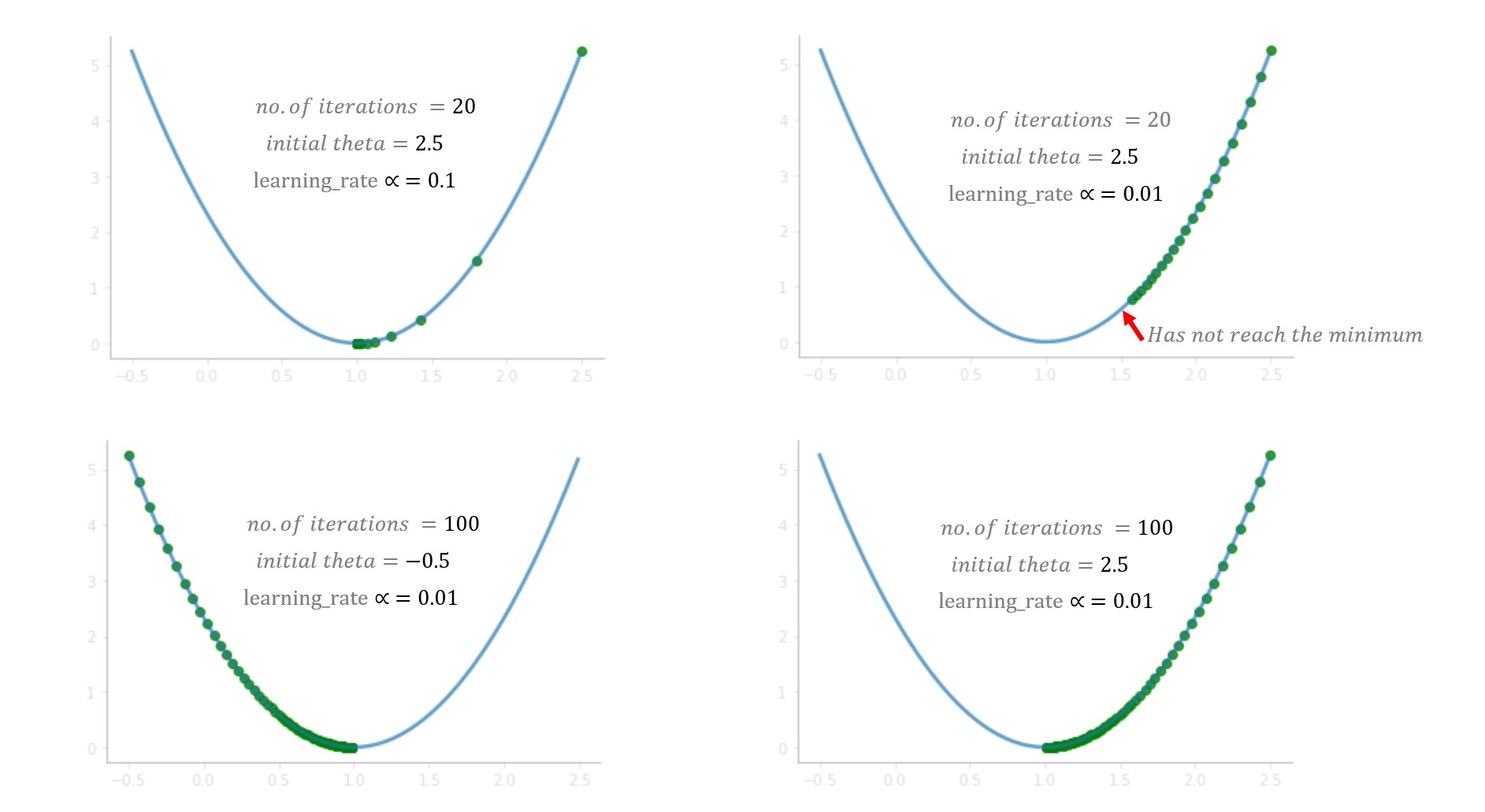
What did you learn from the game? In the beginning, you try with learning rate (alpha)=1 but you fail to reach the minimum, because of the larger steps it overshoots the minimum. In the next game, you try with alpha=0.1, and this time you managed to reach the bottom very safely. what if you had tried with alpha=0.01, well, in that case, you will be gradually coming down but won’t make it to the bottom, 20 jumps are not enough to reach the bottom with alpha=0.01, 100 jumps might be sufficient. while solving a real-world problem, normally alpha between 0.01–0.1 should work fine but it varies with the number of iterations that the algorithm takes, some problems might take 100 or some might even take 1000 iterations.

Based on these factors you can try with different values of alpha. Although tuning alpha value is one of the important tasks in understanding the algorithm I would suggest you look at other parts of the algorithm also like derivative parts, minus sign, update parameters and understand what their individual’s roles are.

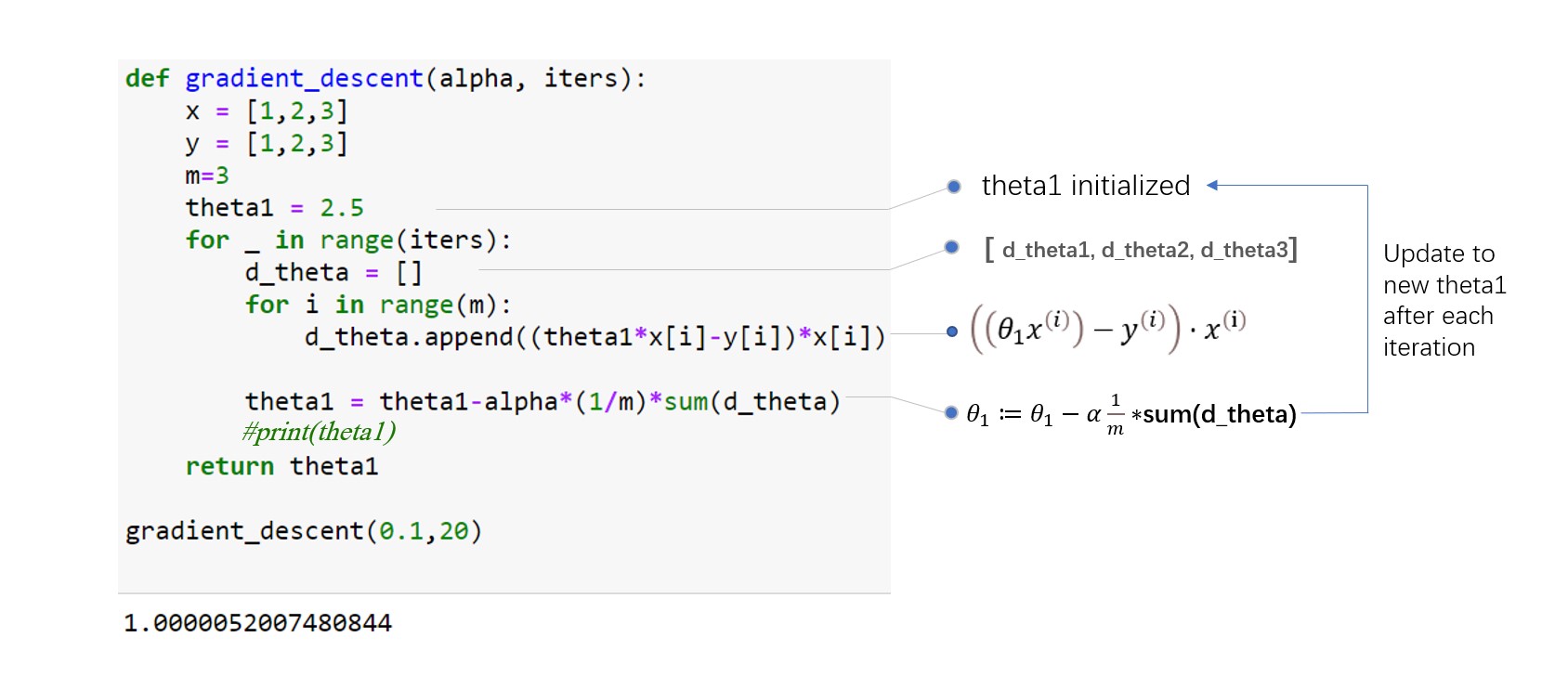
Coding Gradient Descent

Until now we are just using a single parameter to calculate cost function and algorithms. What the cost function looks like and how does the algorithm works when we have two or more parameters? See the figure below for intuitive understanding. Imagine yourself somewhere at the top of the mountain and struggling to get down the bottom of the mountain blindfolded.

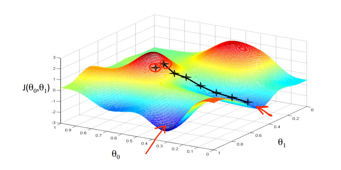
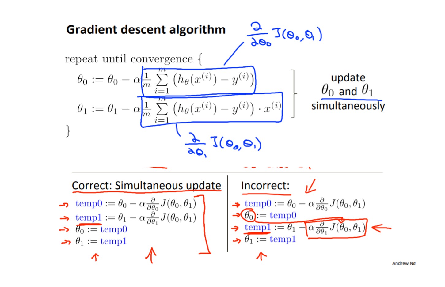
The algorithm working principle is the same for any number of parameters, it’s just that the more the parameters more the direction of the slope. In the previous example of the bowl-shaped curve, we just need to look at the slope of theta1, But now the algorithm needs to look for both directions in order to minimize the cost function. let’s code and understand the algorithm. see the figure below for reference:

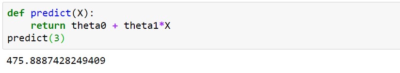
Here we go, Our model predicts 475.88*1000 = $475,880 for the house of size 3*1000 ft square. It’s very close to our prediction that we made earlier at the beginning using our intuition.

Conclusion

As a beginner, it might be a little difficult to grasp all the concepts of linear regression in such a short reading time. I wouldn’t say you know all things about linear regression from this article. The purpose of this article is to make algorithms understandable in the simplest way possible. Please follow the resources’ link below for a better understanding. I hope you enjoyed reading the article. Thanks for reading.

Resources:

code link

https://github.com/ravi235/LinearRegression

Gradient descent mathematics

https://www.youtube.com/watch?v=jc2IthslyzM&ab_channel=TheCodingTrain

Linear Regression Andrew Ng

https://www.youtube.com/watch?v=kHwlB_j7Hkc&t=8s&ab_channel=ArtificialIntelligence-AllinOne

Ravindra Sah 08 Dec 2020