kNN Algorithm – An Instance-based ML Model to Predict Heart Disease

Introduction

Instance-based learning is an important aspect of supervised machine learning. It is a way of solving tasks of approximating real or discrete-valued target functions. The modus operandi of this algorithm is that the training examples are being stored and when the test example is fed, the closest matches are being found. Instance-based learning is referred to as memory-based learning. Examples of this mode of learning are kNN, RBF (Radial basis function) networks, and kernel machines. In this article, we shall discuss kNN with practical implementation.

kNN Algorithm

It is a supervised learning algorithm and is used for both classification tasks and regression tasks. kNN is often referred to as Lazy Learning Algorithm as it does not do any work until it knows what exactly needs to be predicted and from what type of variables. It is a very efficient cross-validation tool, for many users, it is an intelligible learning method, kNN supports both explanation and training, and it can use any distance metric.
Disadvantages associated with memory-based learning are the curse of dimensionality, run time cost scales with training set size, large training sets do not fit into memory, and predicted values in case of regression are not continuous.

Basis of kNN Algorithm Classification

1. During the training method, it saves the training examples.
2. During prediction time, k training examples are being found among examples (x₁,y₁),….(x_k,y_k) that are closest to the test example x. Then, the most frequent class among those y_i‘s are predicted.

Mathematics behind the kNN Algorithm

Euclidean distance is one of the common metrics used for calculation which in turn is used to find out the kNN and prediction.

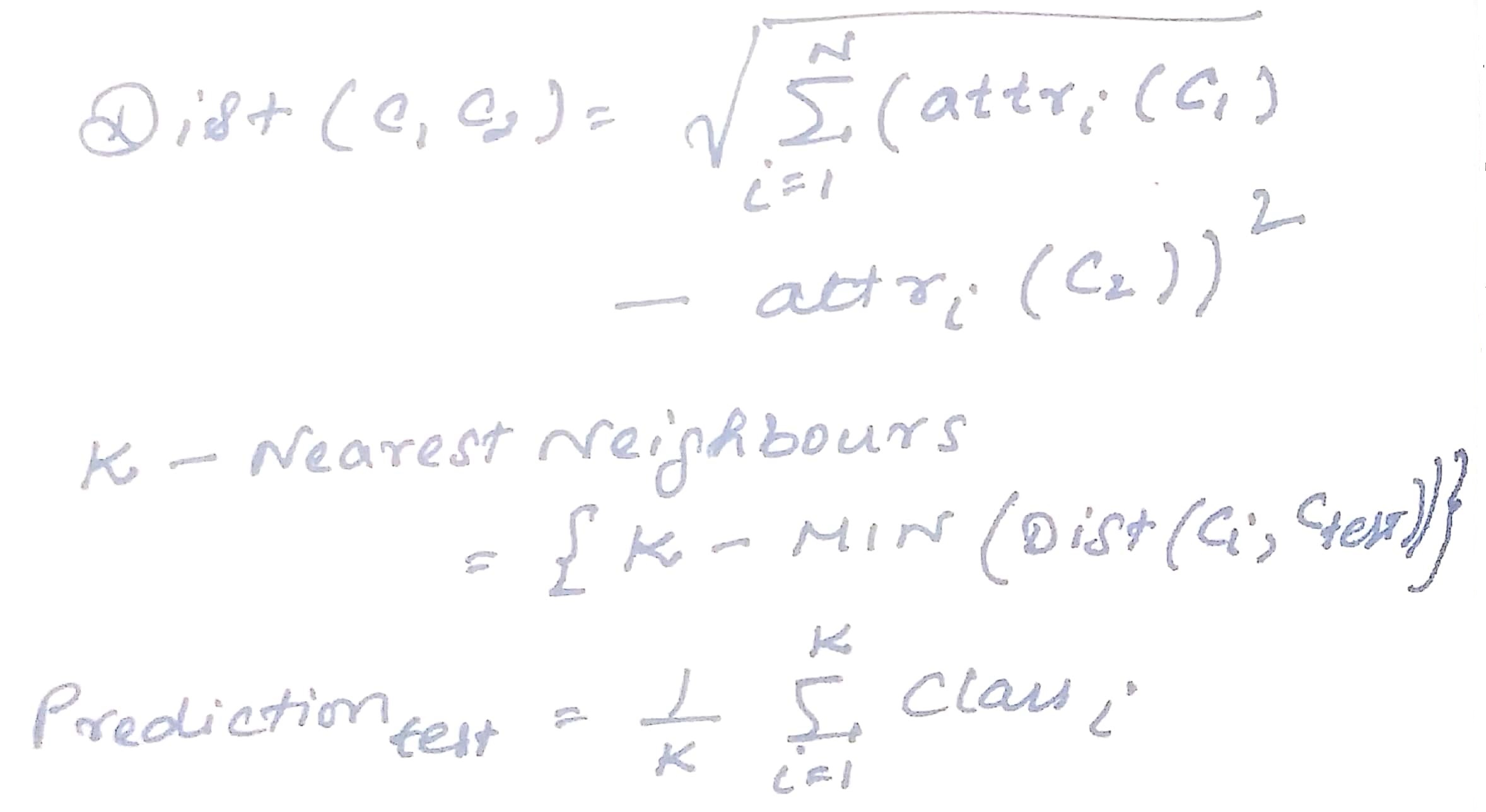
Euclidean distance gives all attributes equal weight when the scale of attributes and differences are similar, and when scale attributes equal range or variance. It assumes spherical classes.

Significance of k and choosing a value of k

‘k’ represents the number of nearest neighbours.

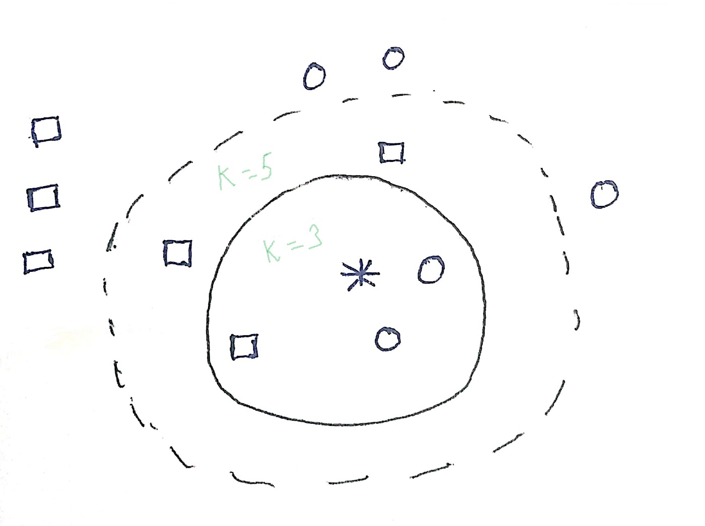
In the above image, we could see some circles and some squares which are the classifications. The asterisk is the test sample which either gets classified under circle or under the square. If k=3, an asterisk is assigned to the circle as there are 2 circles and 1 square. In another instance, if k=5, an asterisk is classified under square as there are 3 squares and 2 circles. In this way, kNN classification is done.  The value of ‘k’ needs to be carefully chosen and the effects of too large and too small a value of ‘k’ have been outlined below

Choosing a large value of K

1. Less sensitive to noise especially noise
2. Better probability estimates for discrete classes
3. Larger training sets allow large values of k

Choosing a smaller value of k

1. Captures fine structure of problem space better
2. Necessary with small training sets
An important aspect of this algorithm is that as the training set approaches infinity, and k grows bigger, kNN becomes Bayes optimal.
The difference between choosing different values of k has been illustrated in the following images

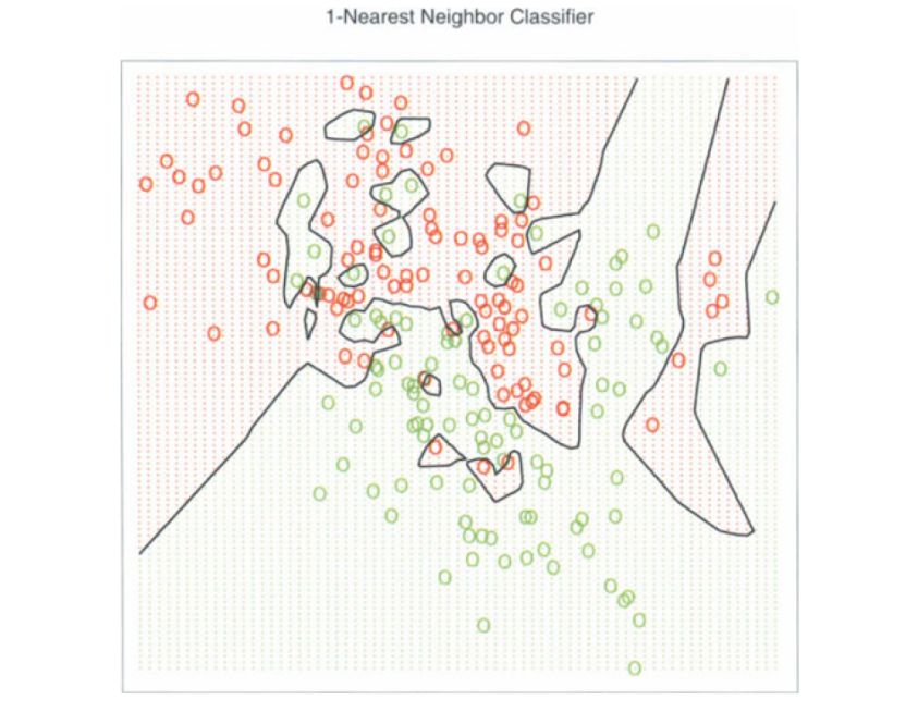
Image 1

Image 2

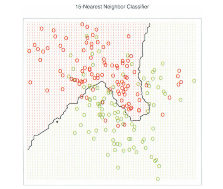
A balance between a large k and a small k needs to be made carefully. As the trade-off between small and large k can be difficult, there exist two approaches that can facilitate the trade-off. These are-

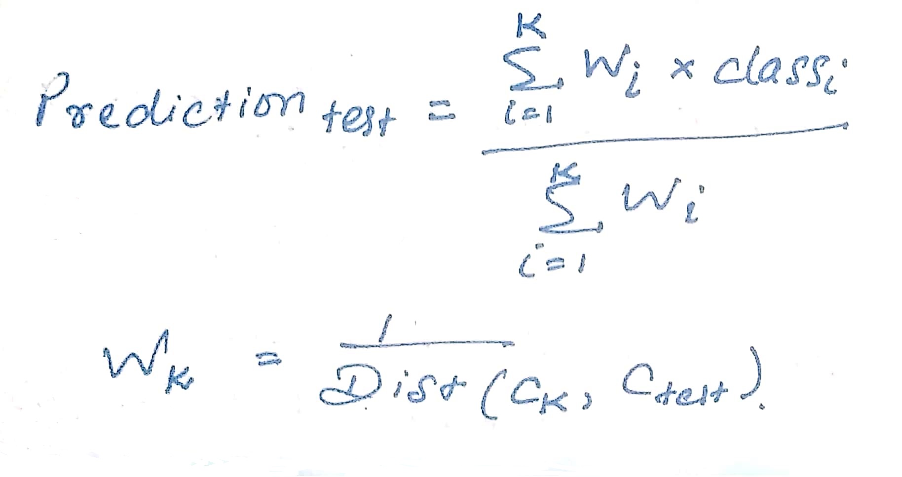
1) Distance weighted kNN

2) Locally weighted averaging

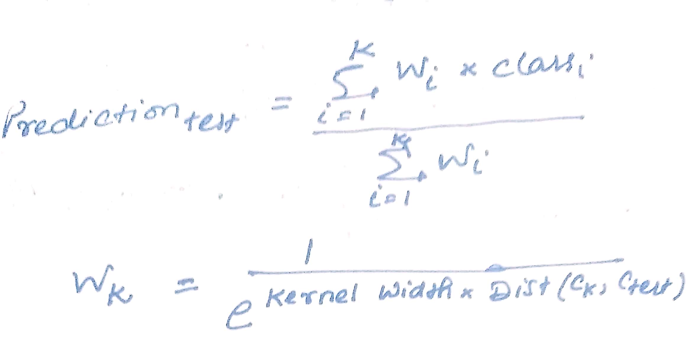
Kernel width controls the size of the neighborhood that has a large effect on values.

Weighted Euclidean Distance

As we have known that Euclidean Distance assumes spherical classes. Now, some questions arise as follows-
a) Cases when classes are not spherical.
b) Cases when attributes are more or less important compared to that of others.
c) Cases when attributes have more or less noise compared to that of others.
Weighted Euclidean Distance is the answer to all these cases. 

Large weights imply attribute is more important, small weights imply attribute is less important, and zero weights imply attribute is immaterial. Weights make kNN more effective in the case of axis parallel elliptical classes.

Industrial application of kNN algorithm
1. Recommender system – Amazon and Flipkart recommend products through targeted marketing tools recommend products based on our search history and likings that we are most likely to buy
2. Concept search – Searches semantically similar documents. With data getting generated every second, each document of data could contain potential concepts. Image recognition, handwriting recognition, and disease classification are important concept searches.

kNN algorithm using python heart disease dataset
Let us now develop an algorithm using kNN to find out the people with heart disease and those without heart disease in the heart disease dataset.

numpy as np
import pandas as pd
import matplotlib.pyplot as plt

First let us start by importing numpy, pandas, and matplotlib.pyplot packages.

df=pd.read_csv('heart.csv')

df is the dataframe where dataset ‘heart’ is loaded.

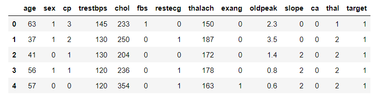
df.head()

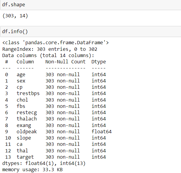
df.shape
df.info()

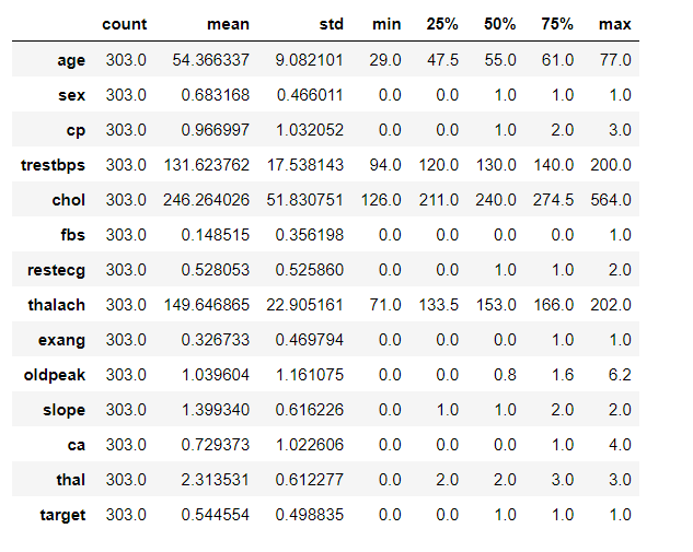
df.describe().T

df.isnull().sum()

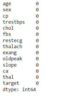
After the loading of the dataset, we have used the head() function to read the first 5 rows of the dataset, shape function is used to find the numbers of rows and columns, in this case, it is 303 rows and 14 columns, info() function gives us information on the data types, columns, null value counts, memory usage, etc. Then, describe() function has been used to generate the descriptive statistics of the dataset. T is for transposing index and columns of the df dataframe. To be sure that the dataset is a clean one, we used the isnull() function and found out that there is no null value. Let us code further

import seaborn as sns
sns.pairplot(df,hue='target')

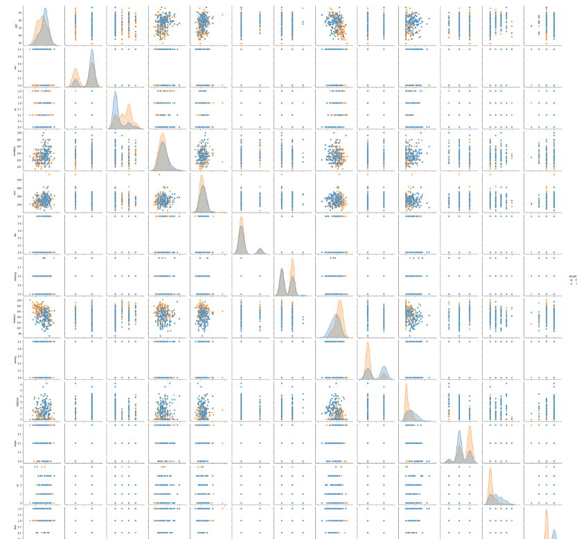
We have imported the seaborn library for data visualization based upon matplotlib and created a pairwise plot. The pairwise plot helps in creating scatterplots for joint relationships and histograms for univariate distribution. Let us further analyze the dataset

plt.figure(figsize=(14,12))
sns.heatmap(df.corr(), annot=True,cmap ='RdYlGn') 

 

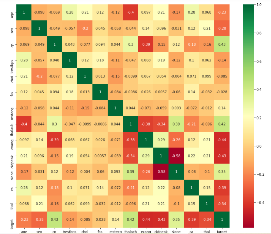
To find the relationship between 2 quantities, we have used Pearson’s correlation coefficient which would also measure the strength between the association of 2 variables. Furthermore, we have used a heatmap to generate a 2-dimensional representation of information using colors. Now, we come to the important part of modeling our data which would give us the power of prediction.

from sklearn.preprocessing import StandardScaler
X =  pd.DataFrame(StandardScaler().fit_transform(df.drop(['target'],axis = 1),),
        columns=['age', 'sex', 'cp', 'trestbps', 'chol','fbs', 'restecg', 'thalach','exang','oldpeak','slope','ca','thal'])
X.head()

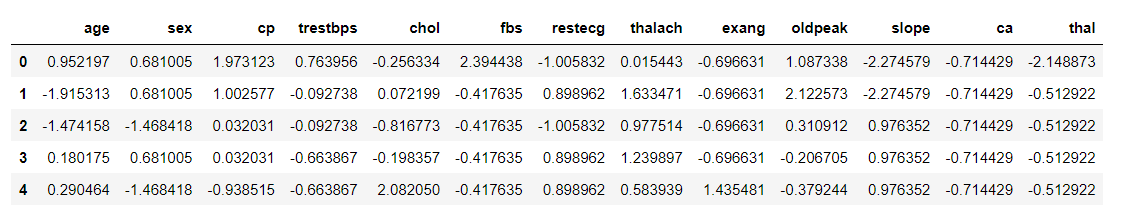
We have imported standard scaler from scikit-learn machine learning library software. Scaling the data is important for kNN as bringing all the features to the same scale is recommended for applying distance-based algorithms.

X = df.drop('target',axis=1).values
y = df['target'].values

from sklearn.model_selection import train_test_split
X_train,X_test,y_train,y_test = train_test_split(X,y,test_size=0.35,random_state=5)

from sklearn.neighbors import KNeighborsClassifier

neighbors = np.arange(1,14)
train_accuracy =np.empty(len(neighbors))
test_accuracy = np.empty(len(neighbors))

for i,k in enumerate(neighbors):
         knn = KNeighborsClassifier(n_neighbors=k)
    knn.fit(X_train, y_train)
    train_accuracy[i] = knn.score(X_train, y_train)
    test_accuracy[i] = knn.score(X_test, y_test)

plt.title('k-NN Varying number of neighbors')
plt.plot(neighbors, test_accuracy, label='Testing Accuracy')
plt.plot(neighbors, train_accuracy, label='Training accuracy')
plt.legend()
plt.xlabel('Number of neighbors')
plt.ylabel('Accuracy')
plt.show()

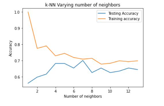
At the outset, we have created numpy arrays for features and targets. Then, we have imported train_test_split from scikit-learn to split the data into train and test datasets. We created a test size of 35%. Then, we have created a classifier using the k-Nearest Neighbors algorithm. Then, we observed the accuracies with different values of k and it can be seen that with k=7, the highest testing accuracy is being shown.

knn = KNeighborsClassifier(n_neighbors=7)

knn.fit(X_train,y_train)

knn.score(X_test,y_test)

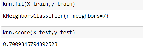
After setting a knn classifier with n_neighbor=7, we fit the model. Then, we get the accuracy score which is 70.09%.

from sklearn.metrics import confusion_matrix,accuracy_score
y_pred = knn.predict(X_test)
confusion_matrix(y_test,y_pred)

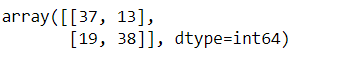
Confusion matrix or an error matrix is the table that identifies true predicted values and is classified as true positive, true negative, false positive, and false negative. Through the crosstab method of pandas, it would be more clear.

pd.crosstab(y_test, y_pred, rownames=['True'], colnames=['Predicted'], margins=True)

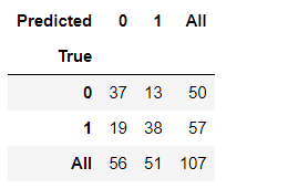
In the above output, 0 refers to the absence of heart disease and 1 refers to the presence of heart disease. 37 subjects are 0~0 means true negative; 38 subjects are 1~1 means true positive; 13 subjects are 0~1 means false positive, and 19 subjects are 1~0 means false negative. That means out of 107 samples, 75 have been classified correctly and the rest have been misclassified. Let’s get the complete classification report

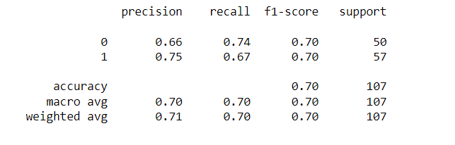
from sklearn.metrics import classification_report
print(classification_report(y_test,y_pred))

Interpretation and observation of the kNN model

The model had an accuracy score of 70.09% where 37 subjects turned out to be true negative; 38 subjects turned out to be true positive; 13 subjects turned out to be falsely positive, and 19 subjects turned out to be false negative. So, out of 107 samples, 75 have been classified correctly and the rest have been misclassified. This model would enable us to correctly classify heart disease and healthy heart to the tune of 70%.

Conclusion

kNN algorithm is a useful supervised learning algorithm not only for recommender systems but also for classifying diseases. This algorithm can help in enabling clinicians to correctly diagnose the presence or the absence of disease; marketing analysts to understand the pattern of consumer behavior and important concept searches.

Image Source-

1. Image 1: https://books.google.co.in/books?id=yPfZBwAAQBAJ&printsec=frontcover&dq=Hastie,+Tibshirani,+Friedman+2001&hl=en&newbks=1&newbks_redir=0&sa=X&ved=2ahUKEwjl0OiihJzzAhU-gtgFHftIAjsQ6AF6BAgHEAI#v=onepage&q=Hastie%2C%20Tibshirani%2C%20Friedman%202001&f=false
2. Image 2: https://books.google.co.in/books?id=yPfZBwAAQBAJ&printsec=frontcover&dq=Hastie,+Tibshirani,+Friedman+2001&hl=en&newbks=1&newbks_redir=0&sa=X&ved=2ahUKEwjl0OiihJzzAhU-gtgFHftIAjsQ6AF6BAgHEAI#v=onepage&q=Hastie%2C%20Tibshirani%2C%20Friedman%202001&f=false